Sequencing: Working with count data

In this lecture we will introduce the main principles of working with count data, and how to model these using generalized linear models (GLMs). We focus on introducing the concept of generalized linear models, and how to interpret its results. We touch briefly upon statistical inference, providing the main results rather than the theory behind it, such that they can be applied to genomics data analysis.

1 The Poisson distribution

• The Poisson distribution is a typical count distribution that is generally popular and fairly easy to work with. It is defined by a single parameter: its mean \(\mu\). For a Poisson distributed random variable \(Y_i\) with observations \(i \in \{1, \ldots, n\}\), its variance is equal to its mean. That is, if \(Y_i \sim Poi(\mu)\), then \(E(Y_i) = Var(Y_i) = \mu\).
• This immediately shows an important feature of count data: the mean-variance relationship. Indeed, in count data, the variance will always be a function of the mean.
• This is quite intuitive. Consider the following example. You have two bird cages, where in one bird cage there are \(10\) birds, while in the other there are \(100\) birds. You let a sample of people count the number of birds in either one of the cages. It seems unlikely that a person in front of the 10-bird cage would come up with an estimate of \(5\), while it seems quite likely that someone in front of the 100-bird cage would come up with an estimate of \(95\). Even though the difference from the true value is the same, the exact value has an impact on the plausible deviation around it.

set.seed(11)
y1 <- rpois(n=500, lambda=10)
y2 <- rpois(n=500, lambda=100)

par(mfrow = c(1,2))
hist(y1, main="Poisson(10)", breaks=40)
hist(y2, main="Poisson(100)", breaks=40)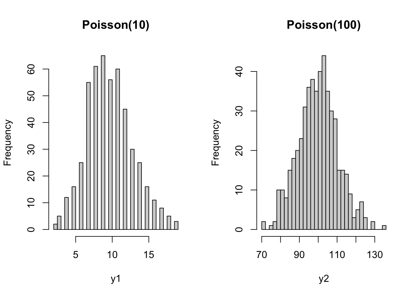

1.1 The Poisson distribution in RNA-seq

• In RNA-seq, technical replicates represent different aliquots of the same sample being sequenced repeatedly. The underlying true expression of a gene can hence safely be assumed to be equal across these technical replicates.
• Marioni et al. (2008) have shown that, for most genes, the distribution of observed gene expression counts across technical replicates follow a Poisson distribution. A small proportion of genes (\(\sim 0.5\%\)) do not follow this Poisson model, however, and actually show evidence for ‘extra-Poisson variation’.

Figure: Technical replication in RNA-seq. Figures from Marioni et al. (2008).

1.2 Relative uncertainty for Poisson distributed random variables

Take a minute to consider the following question:

• Suppose that we have a solid tumor sample from a cancer patient, as well as a sample of surrounding healthy tissue. For each sample, we have three technical replicates at our disposal. Let \(Y_{grt}\) denote the observed gene expression values of gene \(g\) in replicate \(r \in \{1,2,3\}\) from tissue \(t \in \{0,1\}\), where \(t=0\) denotes healthy tissue and \(t=1\) denotes tumoral tissue.
• We then know that the random variables \(Y_{gr0}\) and \(Y_{gr1}\) follow a Poisson distribution, and we would estimate its mean as \(\bar{Y}_{g0} = \frac{1}{3} \sum_{r=1}^3 Y_{gr0}\) and \(\bar{Y}_{g1} = \frac{1}{3} \sum_{r=1}^3 Y_{gr1}\), respectively.
• Similar, for another gene \(k\), we observe \(Y_{krt}\), and estimate \(\bar{Y}_{k0}\) and \(\bar{Y}_{k1}\) correspondingly.
• Now suppose that \(\beta_{k} = \bar{Y}_{k1} / \bar{Y}_{k0} = 5\), but also \(\beta_g = \bar{Y}_{g1} / \bar{Y}_{g0} = 5\), i.e., the two genes have the same average expression ratio (also often called a fold-change) across samples. However, they are differently expressed as \(\bar{Y}_{k1} = 100\), and \(\bar{Y}_{g1} = 10\) (making \(\bar{Y}_{k0} = 20\), and \(\bar{Y}_{g0} = 2\)).
• For which of the two genes is the uncertainty on the expression ratio the highest? In other words, do we trust \(\beta_k\) more or do we trust \(\beta_g\) more?

---

Let’s approximate the uncertainty in \(\beta_g\) and \(\beta_k\) using simulation:

N <- 1e3
beta_g <- beta_k <- vector(length=N)
for(ii in 1:N){
  ygr1 <- rpois(n=3, lambda=10)
  ygr0 <- rpois(n=3, lambda=2)
  ykr1 <- rpois(n=3, lambda=100)
  ykr0 <- rpois(n=3, lambda=20)
  beta_g[ii] <- mean(ygr1) / mean(ygr0)
  beta_k[ii] <- mean(ykr1) / mean(ykr0)
}

par(mfrow=c(1,2), mar=c(4,2,3,1))
hist(beta_g, breaks=seq(0,50,by=1), xlim=c(0,50))
hist(beta_k, breaks=seq(0,50,by=1), xlim=c(0,50))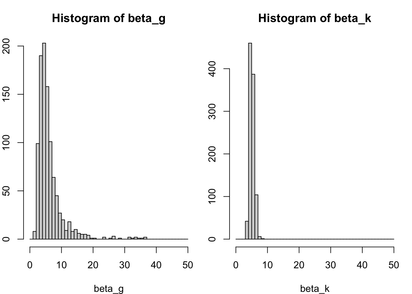

---

We clearly see that the uncertainty on \(\beta_k\) is much lower than on \(\beta_g\). Even though the variance on the counts of gene \(k\) is higher, since its mean is higher and it is distributed as a Poisson variable. How do we explain this?

• We may explain this by considering the relative uncertainty on the mean. Relative uncertainty may be defined as the coefficient of variation \(CV = \frac{\sigma}{\mu}\) (this is, the standard deviation divided by the mean). Indeed, the CV describes the relative deviation of the distribution relative to its mean, where a low CV indicates low dispersion with respect to the mean.
• Calculating the CV shows that the relative uncertainty for gene \(k\) than for gene \(g\), even though the variance on the raw counts is higher for gene \(k\) than for gene \(g\).
• This lower relative uncertainty on the mean then propagates further to a lower uncertainty on the fold-change. This basic result will be essential for understanding the results of a differential expression analysis!

sqrt(100)/100 #CV for gene k

## [1] 0.1

sqrt(10)/10 #CV for gene g

## [1] 0.3162278

2 Modeling count data: Generalized linear models

Just like we have modeled protein abundances in the proteomics module of this course in order to assess differential protein abundance, we can model gene expression counts to identify genes with differences in average expression between groups of samples.

2.1 Why we can(’t) use linear models to model count data

• If we’re using a linear model to model a response \(Y_i\), with \(i \in \{1, \ldots, n\}\) in function of a single covariate \(X_i\), the linear model can be defined as follows:

\[ \left\{ \begin{array}{ccc} Y_i & = & \beta_0 + \beta_1 X_i + \epsilon_i \\ Y_i | X_i & \sim & N(\beta_0 + \beta_1 X_i, \sigma^2 \mathbf{I}). \end{array} \right. \]

• Or, equivalently, we’ve seen we can write it in matrix form as \[ \left\{ \begin{array}{ccc} Y_i & = & \mathbf{X}^T_i \beta + \epsilon_i \\ Y_i | \mathbf{X}_i & \sim & N(\mathbf{X}^T_i \beta, \sigma^2 \mathbf{I}), \end{array} \right. \] where \(\mathbf{X}\) now represents our \(n \times p\) design matrix, with row \(i\) corresponding to observation \(i\).

---

• The variance-covariance matrix of \(\mathbf{Y}\) is assumed a diagonal matrix with \(\sigma^2\) on the diagonal elements and zero everywhere else. This means that the data points are uncorrelated, and that every observation has the same variance \(\sigma^2\), also referred to as homoscedasticity.
• The latter doesn’t hold for count data, due to the mean-variance relationship. This makes linear models, in its basic form, unsuitable to model count data.
• In addition, count data are non-negative, while there are no such constraints in the standard linear model to make sure that our estimates will be non-negative. Indeed, \(\hat{Y}_i = \mathbf{X}^T_i \hat{\beta} \in ] -\infty, \infty[\).

2.2 Generalized linear models

• As the name suggests, generalized linear models (GLMs) extend linear models. In GLMs, we extend two things with respect to the linear model:
  • The conditional distribution of the response variable \(Y_i | X_i\) can be assumed to follow any distribution that belongs to the exponential family of distributions, which includes the Gaussian but also other commonly known distributions, such as the Binomial, Gamma and Poisson distribution.
  • The linear model assumed a linear relationship between \(Y_i\) and \(X_i\), since we assumed that \(E(Y_i | X_i) = \mathbf{X}^T_i \beta\). In GLMs, we will allow a link function \(g()\) that links the conditional mean to the covariates. Hence, in GLMs we have that \(g(E(Y_i | X_i)) = \mathbf{X}^T_i \beta\). Note that each family has got a canonical link function, which is the identity link function \(g(\mu) = \mu\) for Gaussian, the log link function \(g(\mu) = \log \mu\) for Poisson, or the logit link function \(g(\mu) = \log(\frac{\mu}{1-\mu})\) for Binomial.

2.2.1 A Poisson GLM

• We can define a Poisson GLM as follows \[ \left\{ \begin{array}{ccc} Y_i & \sim & Poi(\mu_i) \\ \log \mu_i & = & \eta_i \\ \eta_i & = & \mathbf{X}^T_i \beta \\ \end{array} \right. \] where \(Y_i\) is the response variable, with mean \(\mu_i\), \(\eta_i\) is the linear predictor, \(\mathbf{X}\) is the \(n \times p\) model matrix and \(\beta\) is the \(p \times 1\) matrix of regression coefficients, where \(n\) is the number of data points and \(p\) the total number of parameters to be estimated.
• It is insightful to compare this model to a linear model where \(Y_i\) is log-transformed. Indeed, in the linear model case, we would be modeling \(E(\log Y_i )\), while in the GLM we are modeling \(\log E(Y_i)\).
• This shows that in the GLM setting we are modeling a transformed version of the expected value, and after retransforming we can interpret the fit in terms of the mean of our response variable. In the transformed linear model, however, we are working with the expected value of a transformed version of our response variable, and we will not be able to interpret the fit in terms of the mean, because \(E( \log Y_i) \ne \log E(Y_i)\). In this specific case, we would have to resort to interpreting changes in terms of a geometric mean.
• Also note that \(\mathbf{X}^T_i \beta \in ]-\infty, \infty[\), while \(Y_i\) must be non-negative \([0, \infty[\). The link function helps with this, since the exponential function transforms any real number to a non-negative number, i.e., \(\exp(\mathbf{X}^T_i \beta) \in [0, \infty[\).

2.2.2 Parameter estimation using maximum likelihood

• In maximum likelihood, we attempt to maximize the likelihood function of the data, under the posited assumptions. The likelihood function is typically parametrized by a limited number of parameters, hence we can find the values of the parameters that maximize the likelihood function.
• We do this by finding the point on the likelihood function where its first derivative equals zero, as this must be a maximum of the function. For non-convex likelihood functions, this may be a local maximum, but for GLMs the likelihood function is convex and therefore the obtained maximum must be the global maximum.

2.2.2.1 Maximum likelihood for a linear model

For linear models, we can derive an equivalent estimator for \(\beta\) using maximum likelihood estimation as we had derived in our recap lecture using least squares estimation. We can define a linear model as

\[ Y_i \sim N(\mu_i, \sigma^2\mathbf{I}) \\ \mu_i = \mathbf{X}_i \mathbf{\beta} \]

The likelihood function of the data is the product of the likelihoods of each datum. Since we are assuming a Gaussian distribution, we use the Gaussian probability density function:

\[ L(\mathbf{Y}; \beta, \sigma) = \prod_{i=1}^n \frac{1}{\sqrt{2 \pi \sigma^2}} \exp \left\{ - \frac{(Y_i - \mathbf{X}_i \beta)^2}{2 \sigma^2} \right\} \]

Log-likelihood function

\[ \ell(\mathbf{Y}; \beta, \sigma) = \sum_{i=1}^n \left\{ -\frac{1}{2} \log(2\pi \sigma^2) - \frac{1}{2\sigma^2} (Y_i - \mathbf{X}_i \beta)^2 \right\} \]

Score function is the derivative of the log-likelihood

\[ S(\mathbf{\beta}) = \frac{\partial \ell(\mathbf{Y}; \beta, \sigma)}{\partial \beta} = \sum_{i=1}^n \frac{1}{\sigma^2} \mathbf{X}_i (Y_i - \mathbf{X}_i \beta) \]

Set to zero and solve

\[ \mathbf{X}^T\mathbf{Y} - \mathbf{X}^T \mathbf{X} \mathbf{\beta} = \mathbf{0} \\ \rightarrow \widehat{\mathbf{\beta}} = (\mathbf{X}^T \mathbf{X})^{-1} \mathbf{X}^T\mathbf{Y} \]

which gives us exactly the same estimator as we had derived using least squares!

2.2.2.2 Maximum likelihood for a generalized linear model

Now that we know how to use maximum likelihood for parameter estimation, we can also apply it to estimate the parameters of a generalized linear model. Let’s try it for the Poisson GLM we have just introduced:

\[ \left\{ \begin{array}{ccc} Y_i & \sim & Poi(\mu_i) \\ \log \mu_i & = & \eta_i \\ \eta_i & = & \mathbf{X}^T_i \beta \\ \end{array} \right. \]

Likelihood function of the Poisson distribution

\[ L(Y_i ; \mu) = \prod_{i=1}^n \frac{e^{-\mu} \mu^{Y_i}}{Y_i!} \]

Log-likelihood function

\[ \ell(Y_i ; \mu) = \sum_{i=1}^n - \mu + Y_i \log(\mu) - \log (Y_i!) \]

Note that the score function is the derivative of the log-likelihood with respect to our parameter of interest, \(\beta\). So let’s first rewrite our log-likelihood as a function of our parameter of interest. We know from the model that \(\mu_i = \exp(\mathbf{X}_i \mathbf{\beta})\).

\[ \ell(Y_i ; \beta) = \sum_{i=1}^n - \exp(\mathbf{X}_i \mathbf{\beta}) + Y_i (\mathbf{X}_i \mathbf{\beta}) - \log (Y_i!) \]

The score function then equals

\[ S(\mathbf{\beta}) = \frac{\partial \ell(\mathbf{Y}; \beta)}{\partial \beta} = \sum_{i=1}^n -\mathbf{X}_i^T \exp(\mathbf{X}_i \mathbf{\beta}) + \mathbf{X}_i^TY_i = -\mathbf{X}^T \exp(\mathbf{X} \mathbf{\beta}) + \mathbf{X}^T \mathbf{Y} \]

Set to zero and solve

\[ \mathbf{X}^T \mathbf{Y} = \mathbf{X}^T \exp(\mathbf{X} \mathbf{\beta}) \]

However, since this is a non-linear equation in \(\beta\), we cannot find a closed-form solution! You may see this more clearly when writing out in non-matrix form

\[ \sum_i \sum_p x_{ip} \exp(x_{ip} \beta_p) = \sum_i \sum_p x_{ip} Y_i. \]

---

• The above derivations show that estimating the parameters of a GLM is much harder as compared to a linear model.
• The iterative reweighted least squares (IRLS) algorithm is usually adopted for fitting GLMs using maximum likelihood. As the name suggests, it is an iterative algorithm, where each data point is reweighted in each iteration according to the assumed mean-variance relationship, which is a function of its estimated mean of the previous iteration. Indeed, observations with high variance will be downweighted and vice versa. IRLS uses the derivative of the score function (i.e., the second derivative of the log-likelihood function) to move into the direction where the first derivative is zero.

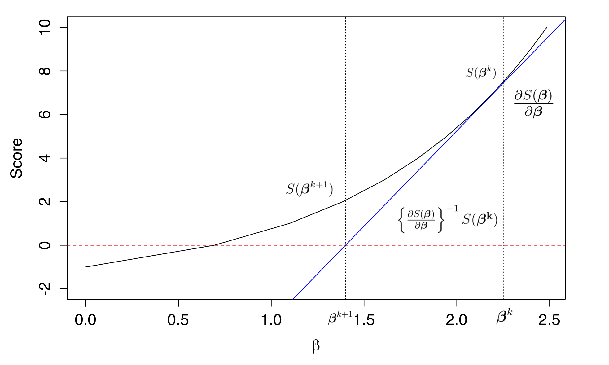Figure: Finding the root of the score function using Newton-Raphson optimization. The Figure shows estimation of a single \(\beta\) parameter. The black solid line is the Score function evaluated at \(\beta\). An initial estimate of \(\beta\) is 2.25, which is represented by the dotted line. The value of the score function of this initial value is \(S(\beta^k)\). The first derivative of the score function at that point, evaluated at \(\beta = 2.25\), is represented by the solid blue line and is given by \(\frac{\partial S(\beta)}{\partial \beta}\). The value of \(\beta\) where the solid blue line crosses zero is the new estimate for \(\beta\), namely \(\beta^{k+1}\) which has a value of 1.4. The difference between \(\beta^{k+1}\) and \(\beta^{k}\) is given by \(\left \{ \frac{ \partial S(\beta)}{ \partial \beta} \right \}^{-1} S(\beta^k)\). This procedure is iterated until a convergence in the \(\beta\) estimate is met.

2.2.3 Generalized linear models in R

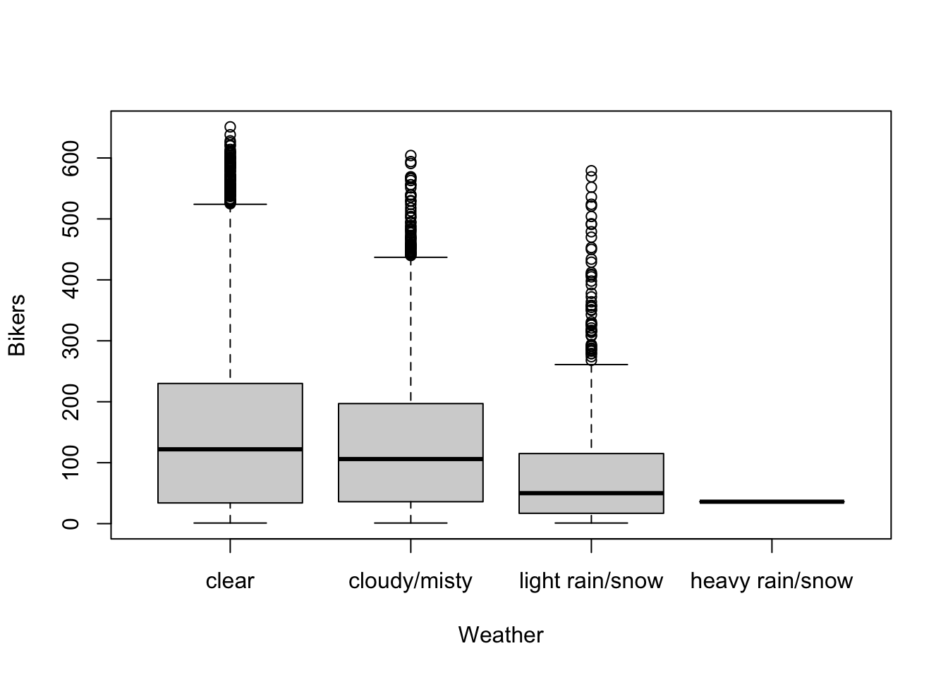
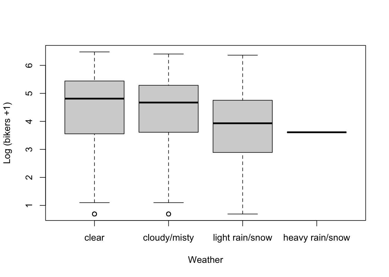
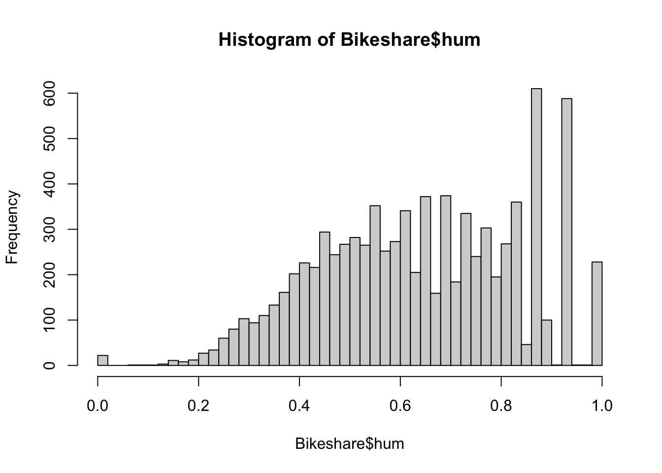
• In order to get familiar with GLMs, we will fit a Poisson GLM in R, using the Bikeshare dataset as part of the ISLR2 package. This dataset records how many bikes were being used from a bike-sharing service, every hour of the day over a full year (365 days).

• Full information of the dataset is provided here. Variables of interest for us are:

  • bikers: Discrete count variable; the number of bikes being used that hour.

  • hum: Continuous variable ranging between 0 and 1; normalized humidity.

  • hr: Categorical variable between 0 and 23; the hour of the day. One could also consider this variable to be numeric and model it as such, but the data exploration will show that’s not appropriate.

  • weathersit: Categorical variable; the weather condition of that hour, with

    1. Clear, Few clouds, Partly cloudy.
    2. Mist + Cloudy, Mist + Broken clouds, Mist + Few clouds, Mist.
    3. Light Snow, Light Rain + Thunderstorm + Scattered clouds, Light Rain + Scattered clouds.
    4. Heavy Rain + Ice Pallets + Thunderstorm + Mist, Snow + Fog.

---

# if ISLR2 isn't installed, install it:
if(!"ISLR2" %in% installed.packages()[,1]){
  install.packages("ISLR2")
}

## Installing package into '/Users/runner/work/_temp/Library'
## (as 'lib' is unspecified)

## 
## The downloaded binary packages are in
##  /var/folders/24/8k48jl6d249_n_qfxwsl6xvm0000gn/T//RtmpmpbBq0/downloaded_packages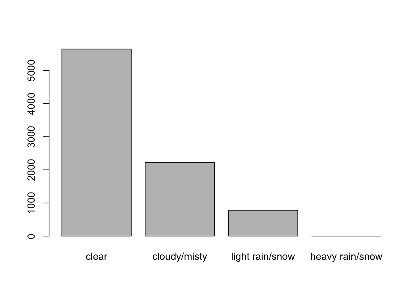

# load and preview the dataset:
data("Bikeshare", package="ISLR2")
head(Bikeshare)

# association with weather on count and log scale
barplot(table(Bikeshare$weathersit))

boxplot(bikers ~ weathersit, data=Bikeshare,
        xlab = "Weather", ylab = "Bikers")

boxplot(log1p(bikers) ~ weathersit, data=Bikeshare,
        xlab = "Weather", ylab = "Log (bikers +1)")

# association with humidity on count and log scale
hist(Bikeshare$hum, breaks=40)

plot(bikers ~ hum, data=Bikeshare, pch=16, cex=1/2,
        xlab = "Humidity", ylab = "Bikers")
loHum <- loess(bikers ~ hum, data=Bikeshare)
xGrid <- seq(0, 1, length=50)
yhat <- predict(loHum, data.frame(hum = xGrid))
lines(x=xGrid, y=yhat, col="red", lwd=3)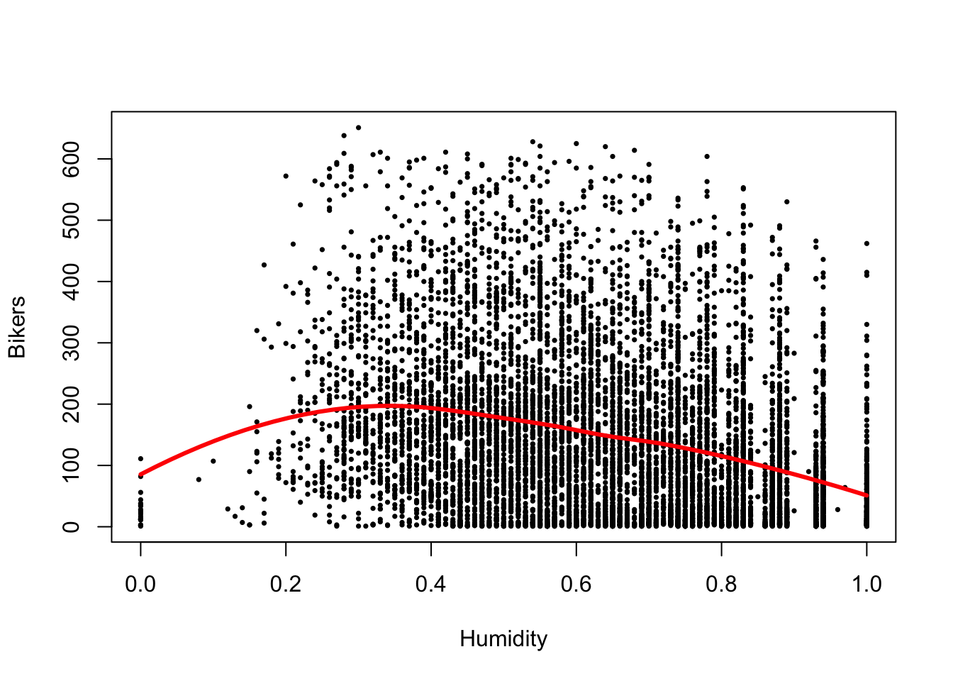

plot(log1p(bikers) ~ hum, data=Bikeshare, pch=16, cex=1/2,
        xlab = "Humidity", ylab = "Log (bikers +1)")
loHum <- loess(log1p(bikers) ~ hum, data=Bikeshare)
xGrid <- seq(0, 1, length=50)
yhat <- predict(loHum, data.frame(hum = xGrid))
lines(x=xGrid, y=yhat, col="red", lwd=3)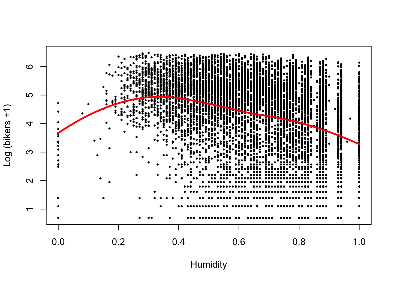

# association with hour on count and log scale
barplot(table(Bikeshare$hr), xlab="Hour of day", ylab="Number of observations")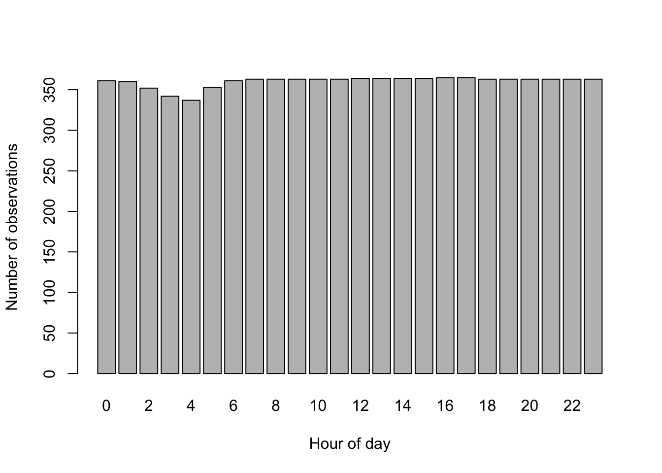

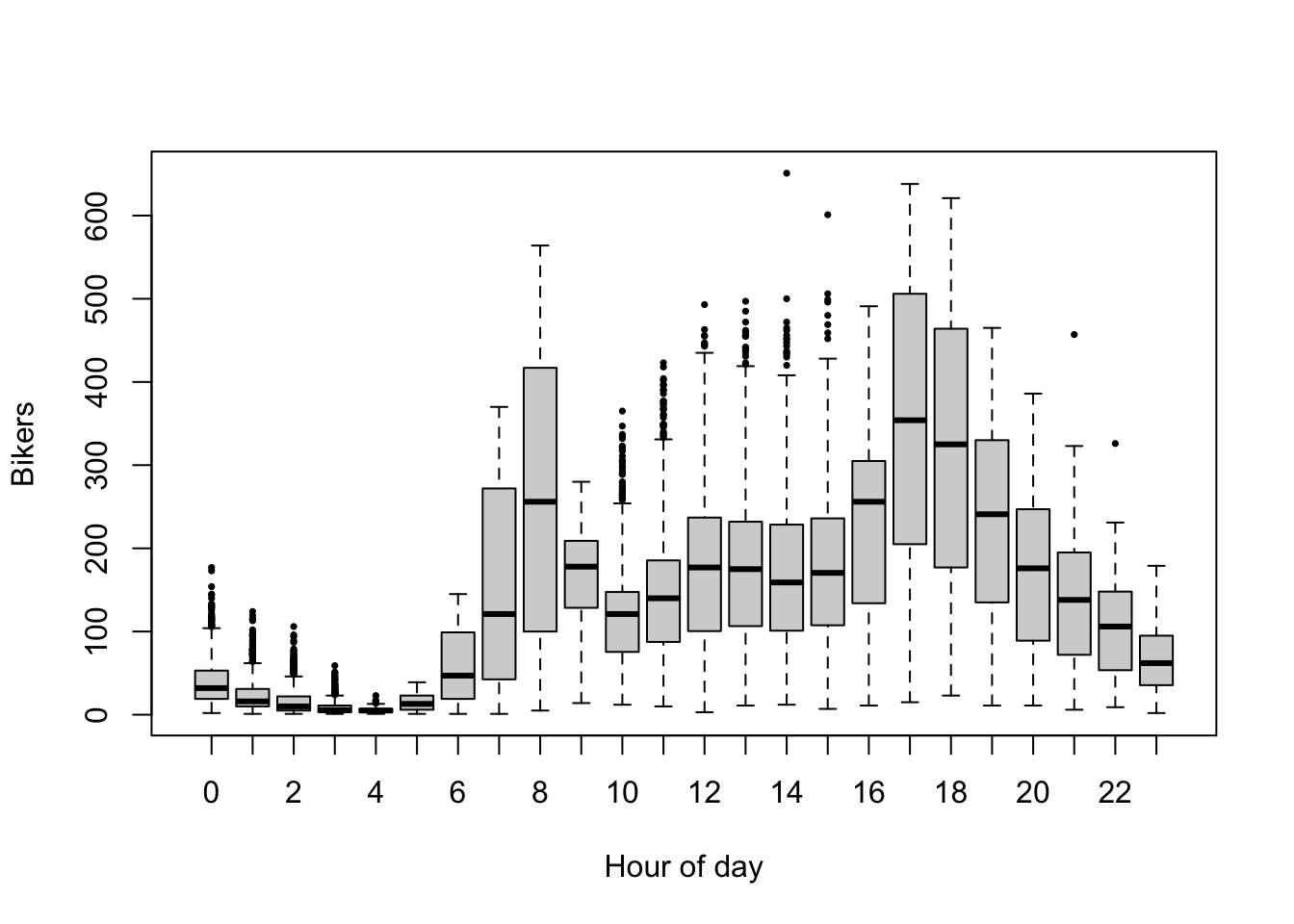
plot(bikers ~ hr, data=Bikeshare, pch=16, cex=1/2,
        xlab = "Hour of day", ylab = "Bikers")

plot(log1p(bikers) ~ hr, data=Bikeshare, pch=16, cex=1/2,
        xlab = "Hour of day", ylab = "Log (bikers +1)")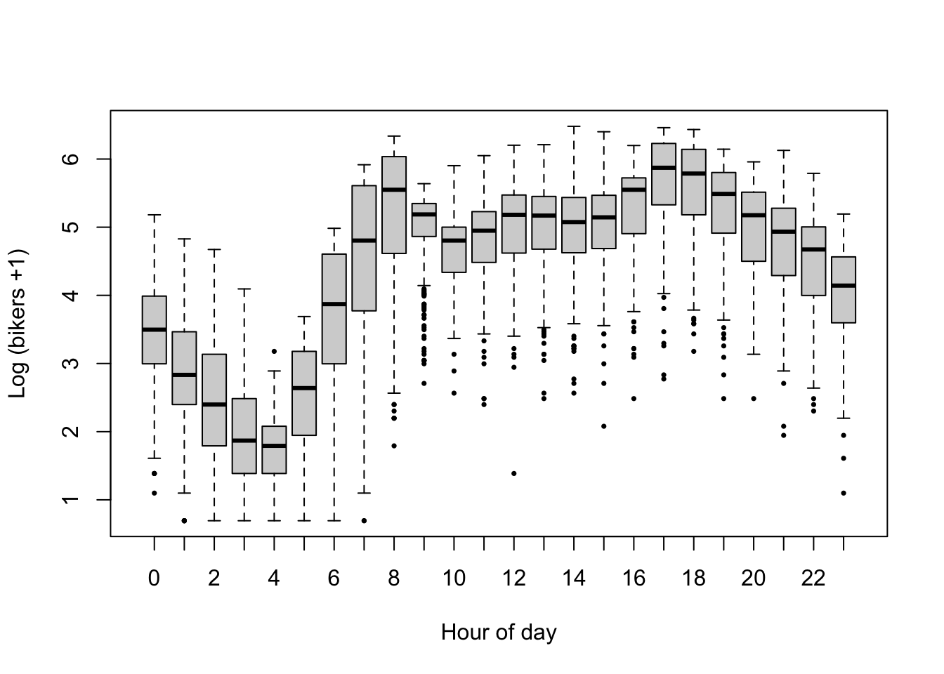

The data exploration shows that

• More bikes are being used in better weather.
• There seems to be a non-linear association between bicycle rentals and humidity, where in both low and high humidity conditions relatively few bikes are used, possibly reflecting very hot and very wet days respectively, while most bikes are being used at moderate humidity.
• Bicycle rental is associated with the hour of the day, however, in a non-linear way, with clear peaks in usage at typical commute hours (6h-8h and 17h-19h). Here, we will add hr as a categorical variable to the model, estimating one parameter for each hour. Note that alternative strategies are possible that may be more efficient, such as incorporating hr as a numerical variable and modeling the non-linearity using a lower number of parameters.
• Disclaimer: Note that there are likely interactions between the variables, which here we will not evaluate as our goal is to introduce a Poisson GLM rather than a full analysis of the Bikeshare dataset. For example, it seems likely that more people commute by bike in good weather, while fewer people will commute by bike in terrible weather. This would motivate an interaction between the variables weathersit and hr.

---

• Below, we fit a Poisson GLM using the glm function. The number of bikers is used as a response variable, which is modeled as a function of weathersit, hum and hr.
• Note that there seems to be a non-linear, though fairly simple, association between our response variable and the humidity. We will therefore add a quadratic and cubic term for humidity to the model. In order to avoid multicollinearity between the linear, quadratic and cubic humidity effects, we will first center the humidity variable and store this in a new variable called humc. This means that when humc=0, this corresponds to the average humidity in the dataset.
• The argument family = "poisson" specifies the Poisson distribution for the response variable and by default the canonical link function, which is the log link, will be used.

Bikeshare$humc <- Bikeshare$hum - mean(Bikeshare$hum)
m <- glm(bikers ~ weathersit + humc + I(humc^2) + I(humc^3) + hr,
         data = Bikeshare,
         family = "poisson")
summary(m)

## 
## Call:
## glm(formula = bikers ~ weathersit + humc + I(humc^2) + I(humc^3) + 
##     hr, family = "poisson", data = Bikeshare)
## 
## Deviance Residuals: 
##      Min        1Q    Median        3Q       Max  
## -23.3408   -4.6201   -0.9922    3.4605   27.4153  
## 
## Coefficients:
##                            Estimate Std. Error  z value Pr(>|z|)    
## (Intercept)                3.893651   0.008083  481.708   <2e-16 ***
## weathersitcloudy/misty    -0.146618   0.002277  -64.401   <2e-16 ***
## weathersitlight rain/snow -0.556153   0.004585 -121.292   <2e-16 ***
## weathersitheavy rain/snow -1.855194   0.166742  -11.126   <2e-16 ***
## humc                       0.091751   0.009233    9.938   <2e-16 ***
## I(humc^2)                 -2.233919   0.029421  -75.929   <2e-16 ***
## I(humc^3)                 -1.823066   0.091428  -19.940   <2e-16 ***
## hr1                       -0.476470   0.012999  -36.654   <2e-16 ***
## hr2                       -0.806959   0.014646  -55.099   <2e-16 ***
## hr3                       -1.433648   0.018842  -76.090   <2e-16 ***
## hr4                       -2.058714   0.024796  -83.027   <2e-16 ***
## hr5                       -1.061695   0.016074  -66.051   <2e-16 ***
## hr6                        0.315691   0.010607   29.761   <2e-16 ***
## hr7                        1.317856   0.009052  145.586   <2e-16 ***
## hr8                        1.830026   0.008653  211.480   <2e-16 ***
## hr9                        1.352135   0.009022  149.871   <2e-16 ***
## hr10                       1.129497   0.009271  121.831   <2e-16 ***
## hr11                       1.308554   0.009102  143.766   <2e-16 ***
## hr12                       1.522234   0.008947  170.131   <2e-16 ***
## hr13                       1.536827   0.008959  171.542   <2e-16 ***
## hr14                       1.499506   0.008999  166.633   <2e-16 ***
## hr15                       1.535043   0.008974  171.062   <2e-16 ***
## hr16                       1.745128   0.008800  198.318   <2e-16 ***
## hr17                       2.140488   0.008565  249.925   <2e-16 ***
## hr18                       2.037740   0.008588  237.279   <2e-16 ***
## hr19                       1.711545   0.008747  195.667   <2e-16 ***
## hr20                       1.393901   0.008976  155.284   <2e-16 ***
## hr21                       1.132543   0.009216  122.895   <2e-16 ***
## hr22                       0.882534   0.009537   92.539   <2e-16 ***
## hr23                       0.481354   0.010207   47.157   <2e-16 ***
## ---
## Signif. codes:  0 '***' 0.001 '**' 0.01 '*' 0.05 '.' 0.1 ' ' 1
## 
## (Dispersion parameter for poisson family taken to be 1)
## 
##     Null deviance: 1052921  on 8644  degrees of freedom
## Residual deviance:  375265  on 8615  degrees of freedom
## AIC: 428362
## 
## Number of Fisher Scoring iterations: 5

2.2.3.1 Interpretation of estimated model parameters

• Remember that the Poisson GLM can be defined as \[ \left\{ \begin{array}{ccc} Y_i & \sim & Poi(\mu_i) \\ \log \mu_i & = & \eta_i \\ \eta_i & = & \mathbf{X}^T_i \beta \\ \end{array} \right. \]

Interpretation of the intercept.

• We will first interpret the intercept, in terms of the average number of bikes being used. Note that the intercept corresponds to hour 0, at good weather (weathersit level 1), and average humidity (humc=0). We will denote the intercept as \(\beta_0\) and its estimate as \(\hat{\beta}_0\). All other coefficients will thus denote a relative change with respect to that reference level.
• The model definition shows that \(\log \mu_i = \mathbf{X}^T_i \mathbf{\beta}\), with \(\mu\) the average number of bikes being used. Since we’re only working with the intercept here, we may write \(\log \mu_i = \beta_0\), and thus \(\mu_i = \exp \beta_0\).
• Plugging in the estimated intercept \(\hat{\beta}_0\), we have \(\exp \hat{\beta}_0 =\) 49.09. In other words, in clear weather with few clouds, at average humidity and at hour 0, an average of 49.09 bikes are being used.

---

Interpretation of weathersitcloudy/misty.

• We will denote this coefficient as \(\beta_1\) and its estimate as \(\hat{\beta}_1\).
• Note that this coefficient defines the difference in linear predictor between weathersit=2 and weathersit=1, all other variables being equal (say, at their reference level). Indeed, define \(\eta_{w2}\) and \(\eta_{w1}\) to denote the linear predictor at weathersit=2, and weathersit=1, respectively. Then, \(\eta_{w2} - \eta_{w1} = (\beta_0 + \beta_1) - \beta_0 = \beta_1\).
• This also means that \(\beta_1 = \log \mu_{w2} - \log \mu_{w1} = \log \frac{\mu_{w2}}{\mu_{21}}\), and thus \(\exp \beta_1 = \frac{\mu_{w2}}{\mu_{21}}\).
• In our case, \(\exp \hat{\beta}_1 =\) 0.86. In words: All other variables being equal, the average number of bikes being used in cloudy/misty weather is \(0.85\) times (or, also, \(85\%\) of) the number of bikes being used in good weather.
• This exercise has shown us that, due to the \(\log\) link function, the parameters in a Poisson GLM cannot be interpreted in terms of absolute differences in averages of the response variable but instead must be interpreted in terms of multiplicative differences!
• If you’re in a meeting and you need a quick way to interpret these parameters, remember that \(exp(1) = 2.72 \approx 3\) and thus a difference of \(1\) (\(-1\)) means the average of the response variable is about three times higher (lower).

---

Interpretation of the humidity effect.

• The humidity effect is a bit more involved to interpret. Due to the quadratic and cubic terms, it is not straight forward to interpret the linear term separately (and the same applies to the quadratic or cubic term); we must interpret both the linear, quadratic and cubic term simultaneously.

• Also due to the higher-order terms, the rate of change in average bikers will not be constant across the range of humidity. We can therefore not interpret the humidity effect using a single number as we’ve done previously.

• We can, however, provide some examples for specific humidity values, along with a visualization of its global effect.

• For example, let’s derive the change in average bikes being used at a humidity that is \(0.2\) above average, versus average humidity.

  For average humidity \(+0.2\) the linear predictor \(\eta_{0.2} = \beta_0 + \beta_4 x_{hum} + \beta_5 x_{hum}^2 + \beta_6 x_{hum}^3 = \beta_0 + \beta_4 0.2 + \beta_5 0.2^2 + \beta_6 0.2^3\).

  For average humidity, the linear predictor \(\eta_{0} = \beta_0 + \beta_4 x_{hum} + \beta_5 x_{hum}^2 + \beta_6 x_{hum}^3 = \beta_0 + \beta_4 0 + \beta_5 0^2 + \beta_6 0^3 = \beta_0\).

  We thus have \(\log \frac{\mu_{0.2}}{\mu_0} = \beta_4 0.2 + \beta_5 0.2^2 + \beta_6 0.2^3\). In our case, \(\log \frac{\hat{\mu}_{0.2}}{\hat{\mu}_0} = 0.091751*0.2 - 2.233919 * 0.2^2 - 1.823066 * 0.2^3 = -0.0856\) and thus \(\frac{\hat{\mu}_{0.2}}{\hat{\mu}_0} = 0.92\). Therefore, at humidity that is \(0.2\) above average, the average number of bikes being used are \(0.92\) times the average number of bikes used at average humidity.

• Just like with linear models, the predict function is extremely helpful when trying to visualize and understand a fitted GLM. In GLMs, the type argument becomes essential when using the predict function. Indeed, by default, estimates are provided on the linear predictor scale: in our case, on the \(\log\) scale. If we’d like predictions on the scale of the response variable, we need to set type="response". You can find more information in the help file using ?predict.glm.

• The visualization shows that the highest number of bikes are being used at around average humidity, with a decreased usage at higher and lower humidities.

humidityGrid <- seq(min(Bikeshare$humc), max(Bikeshare$humc), 
                    length.out = 50)
newDf <- data.frame(weathersit = factor("clear"),
                    hr = factor(8),
                    humc = humidityGrid,
                    "I(humc^2)" = humidityGrid^2,
                    "I(humc^3)" = humidityGrid^3)
yhat <- predict(m, 
                newdata = newDf,
                type = "response")

plot(x = humidityGrid,
     y = yhat,
     type = 'l', lwd=2,
     xlab = "Centered humidity",
     ylab = "Average number of bikers")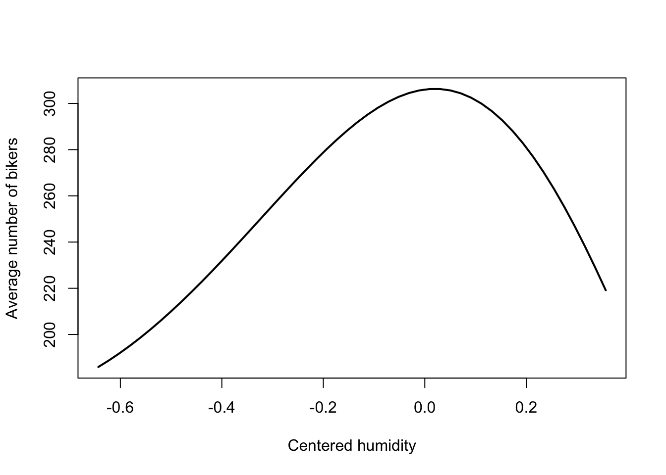

---

Setting up a contrast.

• Suppose we’re interested in whether there are more bikers at (A) maximum humidity (centered humidity value of \(0.357\)), hour 17, in the light rain/snow weather category, versus (B) average humidity, hour 8, in the clear weather category. This requires us to set up a contrast in terms of a linear combination of the model parameters.
• Manually by hand: \[ \log \mu_A = \beta_0 + \beta_2 x_{rainSnow} + \beta_4 x_{hum} + \beta_5 x_{hum}^2 + \beta_6 x_{hum}^3 + \beta_{23} x_{hr17} \\= 3.894 - 0.556 + 0.092 * 0.357 - 2.234 * 0.357^2 - 1.823 * 0.357^3 + 2.140 = 5.143.\\ \log \mu_B = \beta_0 + \beta_{14} x_{hr8} = 3.894 + 1.830 = 5.724.\\ \frac{\mu_A}{\mu_B} = \exp(5.143 - 5.724) = 0.559. \] Thus, at maximum humidity, hour 17, in the light rain/snow weather category the average number of bikers is 56% times the average number of bikers in the average humidity, hour 8, in the clear weather category.
• Manually in R: We can also use matrix multiplication to derive the estimates. We know from our manual calculations above, that the contrast of interest is \((\beta_0 + \beta_2 x_{rainSnow} + \beta_4 x_{hum} + \beta_5 x_{hum}^+ \beta_6 x_{hum}^3 + \beta_{23} x_{hr17}) - (\beta_0 + \beta_{14} x_{hr8})\). We can store this in a contrast matrix, and then multiply it with the coefficients of our model:

L <- matrix(0, 
            nrow = length(coef(m)),
            ncol = 1)
rownames(L) <- names(coef(m))
L["weathersitlight rain/snow",1] <- 1
L["humc",1] <- 0.357
L["I(humc^2)", 1] <- 0.357^2
L["I(humc^3)", 1] <- 0.357^3
L["hr17", 1] <- 1
L["hr8",1] <- -1
L

##                                  [,1]
## (Intercept)                0.00000000
## weathersitcloudy/misty     0.00000000
## weathersitlight rain/snow  1.00000000
## weathersitheavy rain/snow  0.00000000
## humc                       0.35700000
## I(humc^2)                  0.12744900
## I(humc^3)                  0.04549929
## hr1                        0.00000000
## hr2                        0.00000000
## hr3                        0.00000000
## hr4                        0.00000000
## hr5                        0.00000000
## hr6                        0.00000000
## hr7                        0.00000000
## hr8                       -1.00000000
## hr9                        0.00000000
## hr10                       0.00000000
## hr11                       0.00000000
## hr12                       0.00000000
## hr13                       0.00000000
## hr14                       0.00000000
## hr15                       0.00000000
## hr16                       0.00000000
## hr17                       1.00000000
## hr18                       0.00000000
## hr19                       0.00000000
## hr20                       0.00000000
## hr21                       0.00000000
## hr22                       0.00000000
## hr23                       0.00000000

beta <- matrix(coef(m), ncol=1)
exp(t(L) %*% beta) # equals our manual calculation.

##           [,1]
## [1,] 0.5595652

• Using predict in R:

# set up data frames with relevant predictor variables' values.
dfA <- data.frame(weathersit = factor("light rain/snow"),
                    hr = factor(17),
                    humc = 0.357)
dfB <- data.frame(weathersit = factor("clear"),
                    hr = factor(8),
                    humc = 0)

# calculate estimated average number of bikers
yhatA <- predict(m, 
                newdata = dfA,
                type = "response")
yhatB <- predict(m, 
                newdata = dfB,
                type = "response")

yhatA / yhatB # also equal to above.

##         1 
## 0.5595652

---

Exercise: try to derive the change in average number of bikers between (a) humidity of 0.1 above average, clear weather (weathersit=1), at hour 10 and (b) humidity of 0.1 below average, cloudy weather (weathersit=2), at hour 20, using all three methods.

2.3 Statistical inference in GLMs

2.3.1 Wald test and likelihood ratio test

• In our interpretation above we have focussed on deriving changes in the average number of bikers between groups of interest. However, we have not yet tested whether these changes are statistically significant.
• In genomics applications, statistical inference in GLMs is often adopted to test for differential expression between conditions for each gene (e.g., is gene A differently expressed in healthy versus tumoral tissue?), which amounts to testing the null hypothesis of whether a (linear combination of) coefficient(s) equals zero.
• In this course, we will mainly work with two types of statistical tests for GLMs:
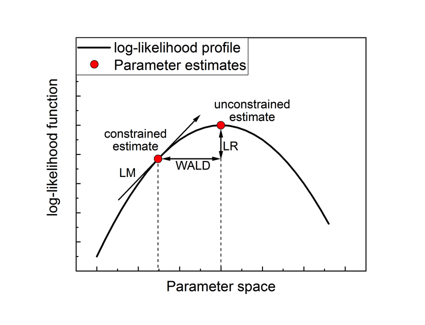
  • Wald test: The Wald test may be viewed as being anaologous to the \(t\)-test we are using in linear models. The Wald test relies on the following asymptotic result \[\hat{\beta} | \beta \sim N (\beta, Var(\hat{\beta}))\]. The Wald test statistic for testing a single parameter \(\hat{\beta}\) \[W = \frac{\hat{\beta}}{\hat{SE}(\hat{\beta})} \sim N(0,1) | H_0\] or, equivalently, letting \(\mathbf{C}\) denote the \(1 \times p\) contrast matrix denoting the contrast for the single parameter \(\beta\) we would like to test, and \(\hat{\Sigma}_{\hat{\beta}}\) the \(p \times p\) variance-covariance matrix of the parameters, \[W = \mathbf{C}\hat{\beta} (\mathbf{C} \hat{\Sigma}_{\hat{\beta}} \mathbf{C}^T)^{-1} \hat{\beta}^T \mathbf{C}^T \sim \chi^2_1 | H_0.\] The null and alternative hypothesis can therefore in general be written as \[ H_0: \mathbf{C} \beta = 0\] \[ H_1: \mathbf{C} \beta \ne 0\] If \(c \ge 1\) contrasts are tested, then the test statistic \(W \sim \chi^2_c | H_0\), provided that the \(c\) contrasts are linearly independent (i.e., the contrast matrix is full rank).
  • Likelihood ratio test: The likelihood ratio test (LRT) measures the discrepancy in log-likelihood between our current model (sometimes also referred to as full model) and a reduced model (sometimes also referred to as null or alternative model). The reduced model must be nested in (and therefore of lower dimension as compared to) the full model. While adding more covariates will always explain more variability in our response variable, the LRT tests whether this is actually significant. For example, in the example of gene differential expression between healthy versus tumoral tissue, the full model could be a GLM where the mean is modeled according to an intercept and a tissue indicator variable (healthy / tumoral), while the alternative model could be a GLM with just an intercept. Indeed, if the gene is similarly expressed between healthy and tumoral tissue, the log-likelihood of the alternative model will decrease only a little as compared to the full model. As the name suggests, the likelihood ratio test assesses whether the ratio of the log-likelihoods provides sufficient evidence for a worse fit of the alternative versus full model \[L = 2 \left\{ \ell(\hat{\beta}_{full}) - \ell(\hat{\beta}_{alternative}) \right\}.\] Asymptotically, under the null hypothesis it can be shown that \[ L \sim \chi_c^2 | H_0, \] with \(c\) the number of parameters dropped in the alternative model versus the full model. If we again let \(\mathbf{C}\) denote the \(c \times p\) contrast matrix denoting the contrast for the parameters being dropped, the null and alternative hypothesis are as in the Wald test setting: \[ H_0: \mathbf{C} \beta = 0\] \[ H_1: \mathbf{C} \beta \ne 0\] Finally, note that while, in this explanation, I have focussed on reducing a more complex model, but of course the LRT can also be adopted to check whether adding a covariate significantly improves the fit.
• It is important to keep in mind that standard statistical inference theory in GLMs works asymptotically in terms of the sample size. Thus we need many data points in order for the theory to hold in practice. In order for the \(p\)-values to be correct, our parametric (distributional) assumptions as well as the independence assumption, must also hold.
• In bulk RNA-seq, we are often working with a limited number of samples and so we typically do not expect asymptotic theory to hold yet. In single-cell RNA-seq, we often perform several preprocessing steps before calculating \(p\)-values for each gene and so we may be ‘using the data multiple times’. Rather than attaching strong probabilistic interpretations to the \(p\)-values, we therefore advice to view the \(p\)-values simply as useful numerical summaries for ranking the genes for further inspection in genomics applications.

2.3.2 Wald test and likelihood ratio test in R

Let’s use a Wald test and a likelihood ratio test to test whether the average number of bikers differs between a working day or a weekend day, using a simple GLM with only that variable as a covariate. This amounts to testing

\[H_0: \beta_{workingday} = 0\] \[H_1: \beta_{workingday} \ne 0\]

mSimple <- glm(bikers ~ workingday, 
               family = "poisson", 
               data = Bikeshare)
summSimple <- summary(mSimple)
summSimple$coefficients["workingday",]

##     Estimate   Std. Error      z value     Pr(>|z|) 
## 2.352087e-02 1.937241e-03 1.214143e+01 6.370326e-34

# Wald test manually
W <- summSimple$coefficients["workingday", "Estimate"] / summSimple$coefficients["workingday", "Std. Error"]
pval <- 2*(1 - pnorm(W))
W

## [1] 12.14143

pval

## [1] 0

# Wald test through a contrast
C <- matrix(0, nrow=1, ncol=length(coef(mSimple)))
colnames(C) <- names(coef(mSimple))
C[, "workingday"] <- 1
C

##      (Intercept) workingday
## [1,]           0          1

beta <- matrix(coef(mSimple), ncol=1)
Sigma <- vcov(mSimple)

W2 <- C %*% beta %*% solve(C %*% Sigma %*% t(C)) %*% t(beta) %*% t(C)
W2

##          [,1]
## [1,] 147.4143

# note this being equal to
W^2

## [1] 147.4143

pval <- 1-pchisq(W2, df=1)
pval

##      [,1]
## [1,]    0

# finally, we can also read the Wald test result from the summary of the model
summSimple

## 
## Call:
## glm(formula = bikers ~ workingday, family = "poisson", data = Bikeshare)
## 
## Deviance Residuals: 
##     Min       1Q   Median       3Q      Max  
## -16.666  -11.361   -3.026    5.214   30.729  
## 
## Coefficients:
##             Estimate Std. Error z value Pr(>|z|)    
## (Intercept) 4.952243   0.001608 3080.12   <2e-16 ***
## workingday  0.023521   0.001937   12.14   <2e-16 ***
## ---
## Signif. codes:  0 '***' 0.001 '**' 0.01 '*' 0.05 '.' 0.1 ' ' 1
## 
## (Dispersion parameter for poisson family taken to be 1)
## 
##     Null deviance: 1052921  on 8644  degrees of freedom
## Residual deviance: 1052773  on 8643  degrees of freedom
## AIC: 1105815
## 
## Number of Fisher Scoring iterations: 5

mFull <- glm(bikers ~ workingday, 
               family = "poisson", 
               data = Bikeshare)

mReduced <- glm(bikers ~ 1, 
               family = "poisson", 
               data = Bikeshare)

# manual LRT
llFull <- logLik(mFull)
llReduced <- logLik(mReduced)

lrt <- as.numeric(2 * (llFull - llReduced))
lrt

## [1] 147.8481

pval <- 1 - pchisq(lrt, df=1)
pval

## [1] 0

# using anova function
anova(mReduced, mFull, test = "Chisq") # note test statistic is identical

2.3.3 Linearly dependent contrasts

Below, we show how one may be able to derive independent contrasts from their contrast matrix for statistical inference. We also show that attempting to use linearly dependent contrasts results in an issue, since the variance-covariance matrix of our contrasts will be singular and therefore non-invertible.

C <- matrix(0, nrow=3, ncol=length(coef(mSimple)))
colnames(C) <- names(coef(mSimple))
C[1, "(Intercept)"] <- 1
C[2, "workingday"] <- 1
C[3,c("(Intercept)", "workingday")] <- c(1,1)
C

##      (Intercept) workingday
## [1,]           1          0
## [2,]           0          1
## [3,]           1          1

# doesn't work because we have a singular matrix
W2 <- try(t(C %*% beta) %*% solve(C %*% Sigma %*% t(C)) %*% C %*% beta)

## Error in solve.default(C %*% Sigma %*% t(C)) : 
##   system is computationally singular: reciprocal condition number = 1.88084e-17

W2 # errrors

## [1] "Error in solve.default(C %*% Sigma %*% t(C)) : \n  system is computationally singular: reciprocal condition number = 1.88084e-17\n"
## attr(,"class")
## [1] "try-error"
## attr(,"condition")
## <simpleError in solve.default(C %*% Sigma %*% t(C)): system is computationally singular: reciprocal condition number = 1.88084e-17>

# identify the linearly independent contrasts
Ct <- t(C)
CtIndep <- Ct[,qr(Ct)$pivot[1:qr(Ct)$rank]]
CIndep <- t(CtIndep)

# try again
W2 <- t(CIndep %*% beta) %*% solve(CIndep %*% Sigma %*% t(CIndep)) %*% CIndep %*% beta
W2

##          [,1]
## [1,] 30686825

2.4 Model deviance, residuals and goodness-of-fit

• In linear models, we often use residuals \(e_i = y_i - \hat{\mu}_i\) to check model assumptions (linearity, homoscedasticity). However, in a GLM setting, we know that the variance of our residuals will depend on the mean, i.e., \(Var(\epsilon_i) = f(\mu_i)\). Using ordinary residuals such as \(e_i\) therefore is no longer appropriate.
• We have seen that the objective function that is used to fit a GLM is the log-likelihood of the data under the posited model. For example, the log likelihood of a Poisson GLM with response variable \(\mathbf{Y}\), with elements \(Y_i, i \in \{1, \ldots, n\}\) and model matrix \(\mathbf{X}\) is \[ \ell(\mathbf{Y}; \beta) = \log \prod_{i=1}^n \left( \frac{\exp (\mathbf{X}_i^T \beta)^{Y_i} \exp( - \exp(\mathbf{X}_i^T \beta))}{Y_i!} \right) = \sum_{i=1}^n \log \left( \frac{\exp(\mathbf{X}_i^T \beta)^{Y_i} \exp( - \exp(\mathbf{X}_i^T \beta))}{Y_i!} \right) \\ = \sum_{i=1}^n Y_i (\mathbf{X}_i^T \beta) - \exp(\mathbf{X}_i^T \beta) - \log Y_i!. \] The estimates \(\hat{\beta}\) are then found by maximizing \(\ell(\beta | \mathbf{Y}, \mathbf{X} )\) with respect to \(\beta\). This is analogous to maximizing a Gaussian likelihood in the linear model setting.
• A goodness-of-fit measure used in the GLM setting is the residual deviance \(D\) (sometimes referred to simply as ‘deviance’), that is twice the difference in log-likelihood between a ‘saturated model’ and the current model. Here, a saturated model, is a model where we fit one parameter per data point and therefore fit the data perfectly, in other words \(\hat{\mu}_i = y_i\). This is, \[ D = 2 * \left\{ \ell(\mathbf{Y}; \beta | \hat{\mu}_i = y_i) - \ell(\mathbf{Y}; \beta | \hat{\mu}_i = \exp(\mathbf{X}_i^T \beta)) \right\}.\]
• From the equation above it becomes clear that the residual deviance is actually a ratio in log-likelihoods and therefore a likelihood ratio test statistic!
• A low residual deviance can thus be interpreted as a model that is fitting the data well, since your current model will be close in log-likelihood to the saturated model. The deviance is a very useful statistic that is also important in statistical inference and model selection, e.g., for testing if a smaller model fits significantly worse than a larger model.
• Finally, a deviance residual \(D_i\) can then be defined as the square root of the contribution of the \(i\)th datum to the residual deviance \[ D_i = sign(Y_i - \exp(\mathbf{X}_i^T \beta)) \sqrt{ 2* \left\{ \ell(Y_i; \beta | \hat{\mu}_i = y_i) - \ell(Y_i; \beta | \hat{\mu}_i = \exp(\mathbf{X}_i^T \beta)) \right\} } \]

---

• Another type of residuals commonly used in a GLM setting are Pearson residuals. A Pearson residual is defined as \[ e_i = \frac{y_i - E(y_i)}{\sqrt{Var(y_i)}},\] and we can see that it has the form of a regular residual such as used in liner models (numerator), but normalized according to the variance of the observed response (denominator), to correct for the mean-variance relationship.

---

• Goodness-of-fit (GOF) analyses serve to assess how well the model actually fits the observed data. One may view the fitting of a GLM as replacing a set of observed data points \(\mathbf{y}\) by a set of fitted values \(\hat{\mathbf{\mu}}\) derived from a model. In general \(\hat{\mathbf{\mu}} \ne \mathbf{y}\) and the question arises as to how well \(\hat{\mathbf{\mu}}\) approximates \(\mathbf{y}\). This naturally raises the question of how much of a discrepancy we believe to be tolerable. Two important discrepancy measures are often used in a GLM setting.
• Note that the residual deviance was a likelihood ratio test statistic between a saturated and our current model. This saturated model actually provides us with a baseline as to how well a model can fit the observed data (even if we know that the saturated model is uninformative for summarizing the data). This motivates a statistical test with
  \(H_0\): The current model provides a similar fit as the saturated model.
  \(H_1\): The current model fits significantly worse than a saturated model.
  
• The residual deviance immediately tests this hypothesis using a likelihood ratio test and is therefore a useful goodness-of-fit measure.
• Another measure of discrepancy is the generalized Pearson \(\chi^2\) statistic \[ X^2 = \sum_{i=1}^n \frac{(y_i - \hat{\mu}_i)^2}{Var(y_i)} = \sum_{i=1}^n e_i^2,\] with \(e_i\) the Pearson residual of observation \(i\).
• Asymptotic theory shows that both the residual deviance \(D \sim \chi^2_{n-p} | H_0\) and \(X^2 \sim \chi^2_{n-p} | H_0\), with \(n\) the number of observations in our dataset (and, hence, the number of parameters fitted in our saturated model), and \(p\) the number of parameters fitted in our current model.

---

Exercise:

• Verify the residual deviance that is reported in the summary of our model above.
• Also check if you can recover the correct deviance and Pearson residuals by calculating them yourself. You can get the correct deviance residuals in R by resid(m, type="deviance") and resid(m, type="pearson").
• Does your model fit significantly worse than a saturated model?

2.5 Overdispersion

• Above we have always assumed that the Poisson distribution is valid for the dataset we have been using. However, we never checked for this.
• As a matter of fact, it often happens that the variance=mean assumption is too stringent for count data. If the variance is larger than the mean, this is referred to as overdispersion. Though much less common, underdispersion happens when the variance is smaller than the mean.
• We can use Pearson residuals to measure overdispersion using the following argument. The Poisson GLM implies that \[ Y_i | X, \hat{\beta} \sim Poi(\hat{\mu}_i),\] with \(\hat{\mu}_i = \exp (\mathbf{X}_i^T \hat{\beta})\). This implies \[ Var(Y_i | X, \hat{\beta}) = \hat{\mu}_i.\] Since the variance is unaffected by addition we may also write \[ Var(Y_i - \hat{\mu}_i | X, \hat{\beta}) = \hat{\mu}_i.\] Which is also equal to \[ Var\left(\frac{Y_i - \hat{\mu}_i}{\sqrt{Var(Y_i)}} | X, \hat{\beta} \right) = \frac{\hat{\mu}_i}{Var(Y_i)}.\] Since we know from the Poisson distribution that \(Var(Y_i) = \hat{\mu}_i\), we have that \[ Var \left(\frac{Y_i - \hat{\mu}_i}{\sqrt{\hat{\mu}_i}} | X, \hat{\beta} \right) = \frac{\hat{\mu}_i}{\hat{\mu}_i}.\] Note that the formulation within the variance at left-hand side of the equation is our definition of Pearson residuals \(E_i\). Thus, if the Poisson assumption holds, we can write \[ Var(E_i | X, \hat{\beta}) = 1,\] which is something we can empirically test using our fitted model. Indeed, if the variance of our Pearson residuals is much larger than \(1\), we are dealing with overdispersion. As a rough rule, I consider overdispersion to be present if this value is larger than \(\sim 1.3\), but this is arbitrary and may depend on the situation (and statistician).

---

• Below, we apply this to the Bikeshare dataset. We will notice that the overdispersion is huge! The p-values and standard errors provided by the model can therefore not be trusted!

ePearson <- resid(m, type="pearson")
n <- nrow(Bikeshare)
p <- length(coef(m))
varPearson <- sum((ePearson^2)) / (n - p)
varPearson # HUGE!

## [1] 42.44815

2.5.1 Remedies to overdispersion

• The presence of overdispersion tells us that the distributional assumption we have been making does not hold. Overdispersion is a common problem, and luckily we have a few available remedies, as in alternative distributions, although choosing between them may not always be trival.
  • The negative binomial (NB) distribution is a popular choice for modeling data that are overdispersed with respect to the Poisson distribution. The NB can be considered as a member of the exponential family and therefore fitted using standard GLM fitting engines. Just like the Poisson distribution, it is a distribution only appropriate for modeling count data. If \[ Y_i \sim NB(\mu_i, \phi), \] then \(E(Y_i) = \mu_i\) and \(Var(Y_i) = \mu_i + \phi \mu_i^2\), with \(\phi \ge 0\) the dispersion parameter. Since \(\phi \ge 0\) the variance of the negative binomial is always larger than that of the Poisson distribution, and in fact is now a quadratic (rather than linear) function of the mean. When \(\phi = 0\), the NB reduces to the Poisson distribution.
  • The quasi-Poisson model is an alternative choice derived using the quasi-likelihood framework developed by Wedderburn (1974). However, only the first two moments (mean and variance) are specified, and all other moments are left unspecified. In particular if model \(Y_i\) using a quasi-Poisson model, then \(E(Y_i) = \mu_i\) and \(Var(Y_i) = \phi \mu_i\), with \(\phi \ge 0\) the (quasi-)dispersion parameter. Again, since \(\phi \ge 0\) the variance of the quasi-Poisson is always larger than that of the Poisson distribution, however, the dispersion parameter here is on the linear scale, and so the mean-variance relationship is still linear as opposed to quadratic in the NB.

---

Below, we fit a negative binomial and quasi-Poisson model in R.

## negative binomial
library(MASS)
mNB <- glm.nb(bikers ~ weathersit + humc + I(humc^2) + I(humc^3) + hr,
         data = Bikeshare)
summary(mNB)

## 
## Call:
## glm.nb(formula = bikers ~ weathersit + humc + I(humc^2) + I(humc^3) + 
##     hr, data = Bikeshare, init.theta = 2.420957542, link = log)
## 
## Deviance Residuals: 
##     Min       1Q   Median       3Q      Max  
## -4.0170  -0.9246  -0.1729   0.5008   5.4746  
## 
## Coefficients:
##                           Estimate Std. Error z value Pr(>|z|)    
## (Intercept)                3.86978    0.03560 108.701  < 2e-16 ***
## weathersitcloudy/misty    -0.15215    0.01753  -8.681  < 2e-16 ***
## weathersitlight rain/snow -0.62708    0.02956 -21.212  < 2e-16 ***
## weathersitheavy rain/snow -1.95785    0.66526  -2.943  0.00325 ** 
## humc                       0.22567    0.06968   3.239  0.00120 ** 
## I(humc^2)                 -1.95867    0.20007  -9.790  < 2e-16 ***
## I(humc^3)                 -0.75361    0.59317  -1.270  0.20391    
## hr1                       -0.47370    0.04968  -9.535  < 2e-16 ***
## hr2                       -0.79592    0.05041 -15.789  < 2e-16 ***
## hr3                       -1.42636    0.05216 -27.346  < 2e-16 ***
## hr4                       -2.04660    0.05478 -37.360  < 2e-16 ***
## hr5                       -1.05264    0.05085 -20.701  < 2e-16 ***
## hr6                        0.32952    0.04909   6.712 1.92e-11 ***
## hr7                        1.33266    0.04868  27.375  < 2e-16 ***
## hr8                        1.86123    0.04862  38.283  < 2e-16 ***
## hr9                        1.38427    0.04877  28.382  < 2e-16 ***
## hr10                       1.14603    0.04900  23.390  < 2e-16 ***
## hr11                       1.32835    0.04913  27.035  < 2e-16 ***
## hr12                       1.54916    0.04934  31.401  < 2e-16 ***
## hr13                       1.56716    0.04951  31.655  < 2e-16 ***
## hr14                       1.53797    0.04960  31.010  < 2e-16 ***
## hr15                       1.57197    0.04961  31.689  < 2e-16 ***
## hr16                       1.78550    0.04947  36.092  < 2e-16 ***
## hr17                       2.19094    0.04924  44.491  < 2e-16 ***
## hr18                       2.08597    0.04911  42.473  < 2e-16 ***
## hr19                       1.75147    0.04890  35.816  < 2e-16 ***
## hr20                       1.41815    0.04883  29.044  < 2e-16 ***
## hr21                       1.14329    0.04875  23.450  < 2e-16 ***
## hr22                       0.89344    0.04879  18.313  < 2e-16 ***
## hr23                       0.49606    0.04891  10.142  < 2e-16 ***
## ---
## Signif. codes:  0 '***' 0.001 '**' 0.01 '*' 0.05 '.' 0.1 ' ' 1
## 
## (Dispersion parameter for Negative Binomial(2.421) family taken to be 1)
## 
##     Null deviance: 26632.4  on 8644  degrees of freedom
## Residual deviance:  9314.9  on 8615  degrees of freedom
## AIC: 93224
## 
## Number of Fisher Scoring iterations: 1
## 
## 
##               Theta:  2.4210 
##           Std. Err.:  0.0374 
## 
##  2 x log-likelihood:  -93161.6150

mean(resid(mNB, type = "pearson")^2) # no more overdispersion!

## [1] 0.9833573

## quasi-Poisson
mQP <- glm(bikers ~ weathersit + humc + I(humc^2) + I(humc^3) + hr,
         data = Bikeshare,
         family="quasipoisson")
# note the dispersion parameter being estimated is equal to our overdispersion diagnostic measure. 
# Indeed, this is the way the dispersion parameter is estimated for the QP!!
summary(mQP) 

## 
## Call:
## glm(formula = bikers ~ weathersit + humc + I(humc^2) + I(humc^3) + 
##     hr, family = "quasipoisson", data = Bikeshare)
## 
## Deviance Residuals: 
##      Min        1Q    Median        3Q       Max  
## -23.3408   -4.6201   -0.9922    3.4605   27.4153  
## 
## Coefficients:
##                           Estimate Std. Error t value Pr(>|t|)    
## (Intercept)                3.89365    0.05266  73.936  < 2e-16 ***
## weathersitcloudy/misty    -0.14662    0.01483  -9.885  < 2e-16 ***
## weathersitlight rain/snow -0.55615    0.02987 -18.617  < 2e-16 ***
## weathersitheavy rain/snow -1.85519    1.08636  -1.708  0.08773 .  
## humc                       0.09175    0.06015   1.525  0.12723    
## I(humc^2)                 -2.23392    0.19169 -11.654  < 2e-16 ***
## I(humc^3)                 -1.82307    0.59568  -3.060  0.00222 ** 
## hr1                       -0.47647    0.08469  -5.626 1.90e-08 ***
## hr2                       -0.80696    0.09542  -8.457  < 2e-16 ***
## hr3                       -1.43365    0.12276 -11.679  < 2e-16 ***
## hr4                       -2.05871    0.16155 -12.744  < 2e-16 ***
## hr5                       -1.06169    0.10473 -10.138  < 2e-16 ***
## hr6                        0.31569    0.06911   4.568 4.99e-06 ***
## hr7                        1.31786    0.05898  22.346  < 2e-16 ***
## hr8                        1.83003    0.05638  32.459  < 2e-16 ***
## hr9                        1.35214    0.05878  23.003  < 2e-16 ***
## hr10                       1.12950    0.06040  18.699  < 2e-16 ***
## hr11                       1.30855    0.05930  22.066  < 2e-16 ***
## hr12                       1.52223    0.05829  26.113  < 2e-16 ***
## hr13                       1.53683    0.05837  26.329  < 2e-16 ***
## hr14                       1.49951    0.05863  25.576  < 2e-16 ***
## hr15                       1.53504    0.05846  26.256  < 2e-16 ***
## hr16                       1.74513    0.05733  30.439  < 2e-16 ***
## hr17                       2.14049    0.05580  38.360  < 2e-16 ***
## hr18                       2.03774    0.05595  36.419  < 2e-16 ***
## hr19                       1.71154    0.05699  30.032  < 2e-16 ***
## hr20                       1.39390    0.05848  23.834  < 2e-16 ***
## hr21                       1.13254    0.06004  18.863  < 2e-16 ***
## hr22                       0.88253    0.06214  14.203  < 2e-16 ***
## hr23                       0.48135    0.06650   7.238 4.94e-13 ***
## ---
## Signif. codes:  0 '***' 0.001 '**' 0.01 '*' 0.05 '.' 0.1 ' ' 1
## 
## (Dispersion parameter for quasipoisson family taken to be 42.44818)
## 
##     Null deviance: 1052921  on 8644  degrees of freedom
## Residual deviance:  375265  on 8615  degrees of freedom
## AIC: NA
## 
## Number of Fisher Scoring iterations: 5

• ver Hoef et al. (2007) provide a useful diagnostic to empirically check whether your data is more amenable to a quasi-Poisson versus a negative binomial distribution.

3 A final note

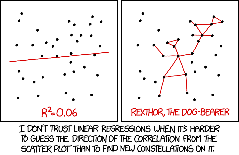
In this lecture, we have introduced GLMs to model data that can be assumed to follow a distribution belonging to the exponential family. We focussed on estimation, interpretation, statistical inference and some model goodness-of-fit diagnostics. We did not consider important topics like model selection, or even whether a GLM is appropriate for your dataset! These are other important topics which, unfortunately, we do not have the bandwidth for to include in this course. Therefore, a final note through an XKCD comic, after finishing this long chapter!

4 References

• Marioni et al. (2008) describe the distribution of gene expression counts across technical replicates, and in addition discuss lane effects in RNA-seq, as well as a comparison between RNA-seq and array-based platforms.
• Wedderburn (1974) introduced the (extended) quasi-likelihood framework.
• The count data chapter of Modern Statistics for Modern Biology by Wolfgang Huber and Susan Holmes handles similar topics also in the context of RNA-seq: https://www.huber.embl.de/msmb/Chap-CountData.html