Recap general linear model

This is part of the online course Statistical Genomics 2021 (SGA21)

1 Breast cancer example

• part of study https://doi.org/10.1093/jnci/djj052)
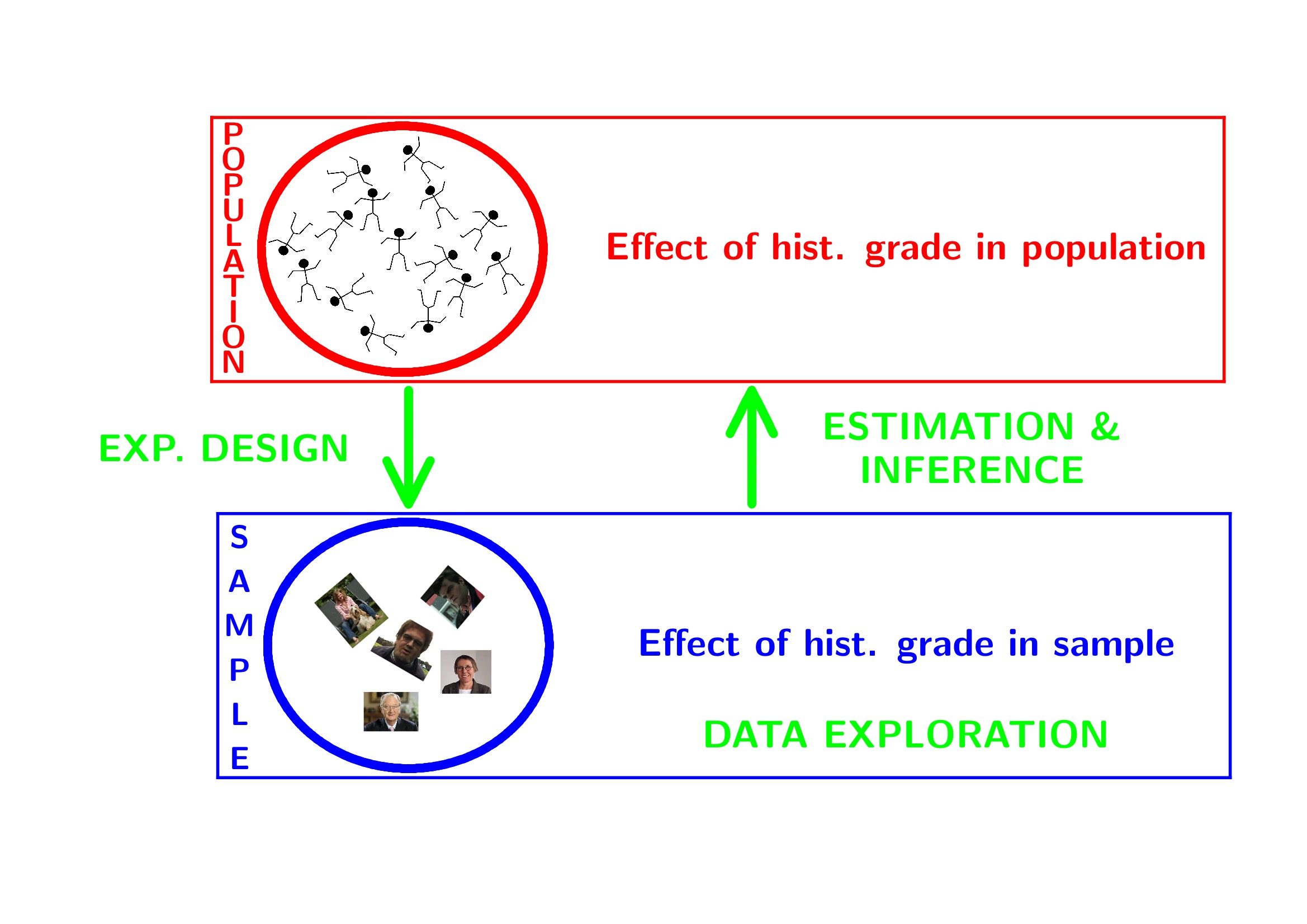
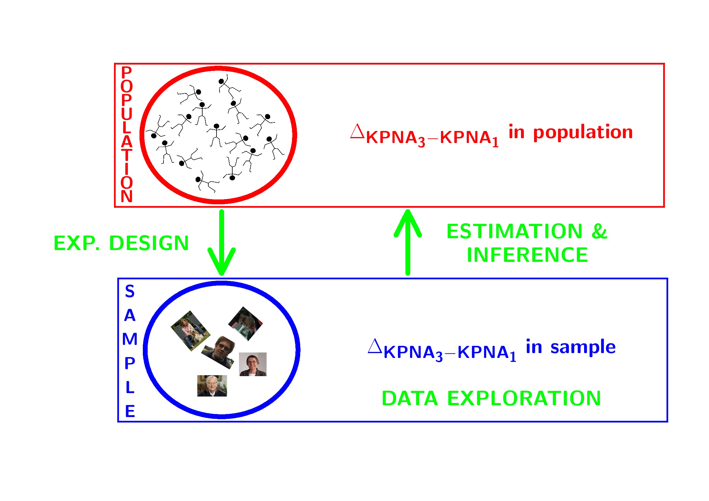
• Histologic grade in breast cancer clinically prognostic. Association of histologic grade on expression of KPNA2 gene that is known to be associated with poor BC prognosis.
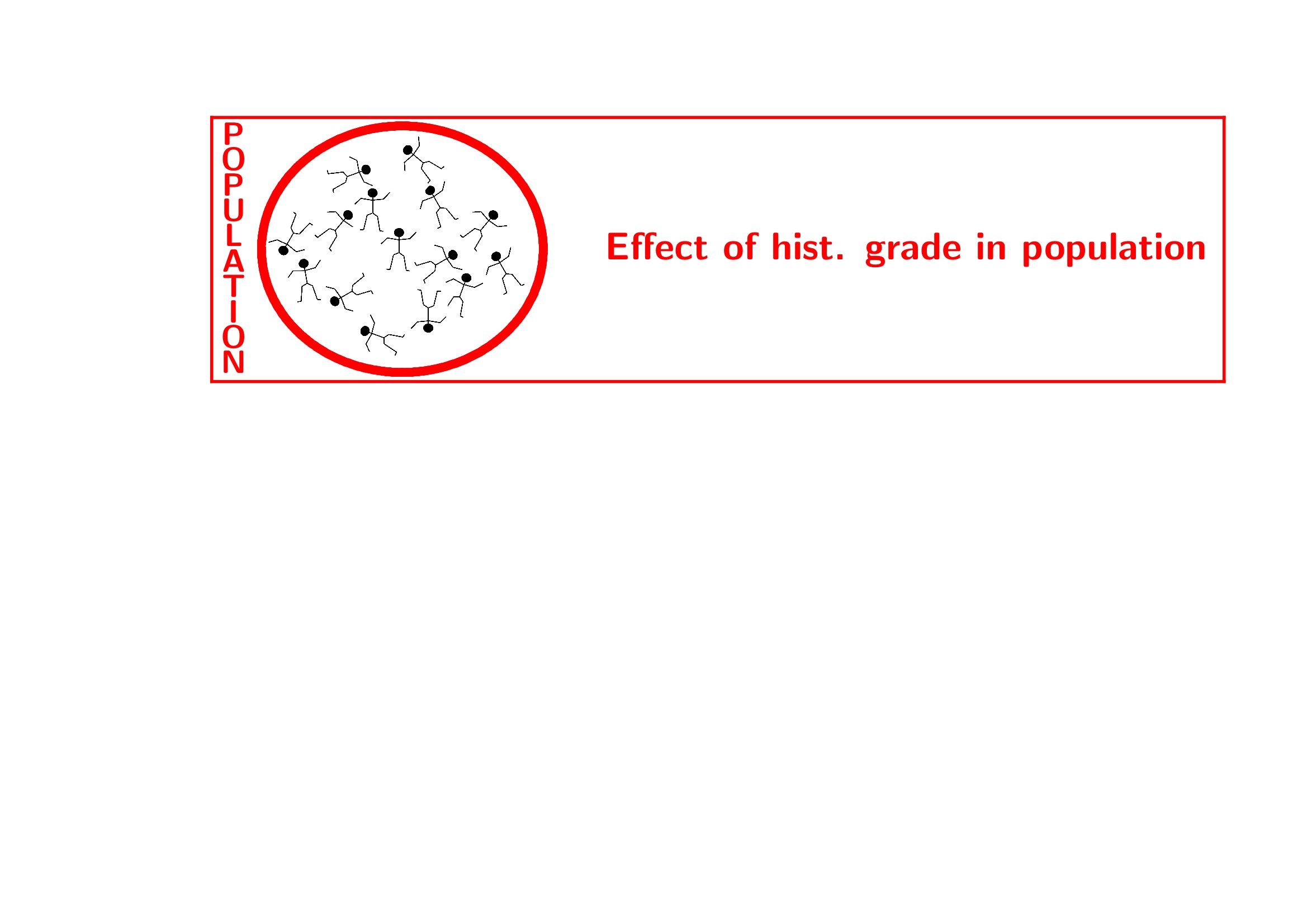
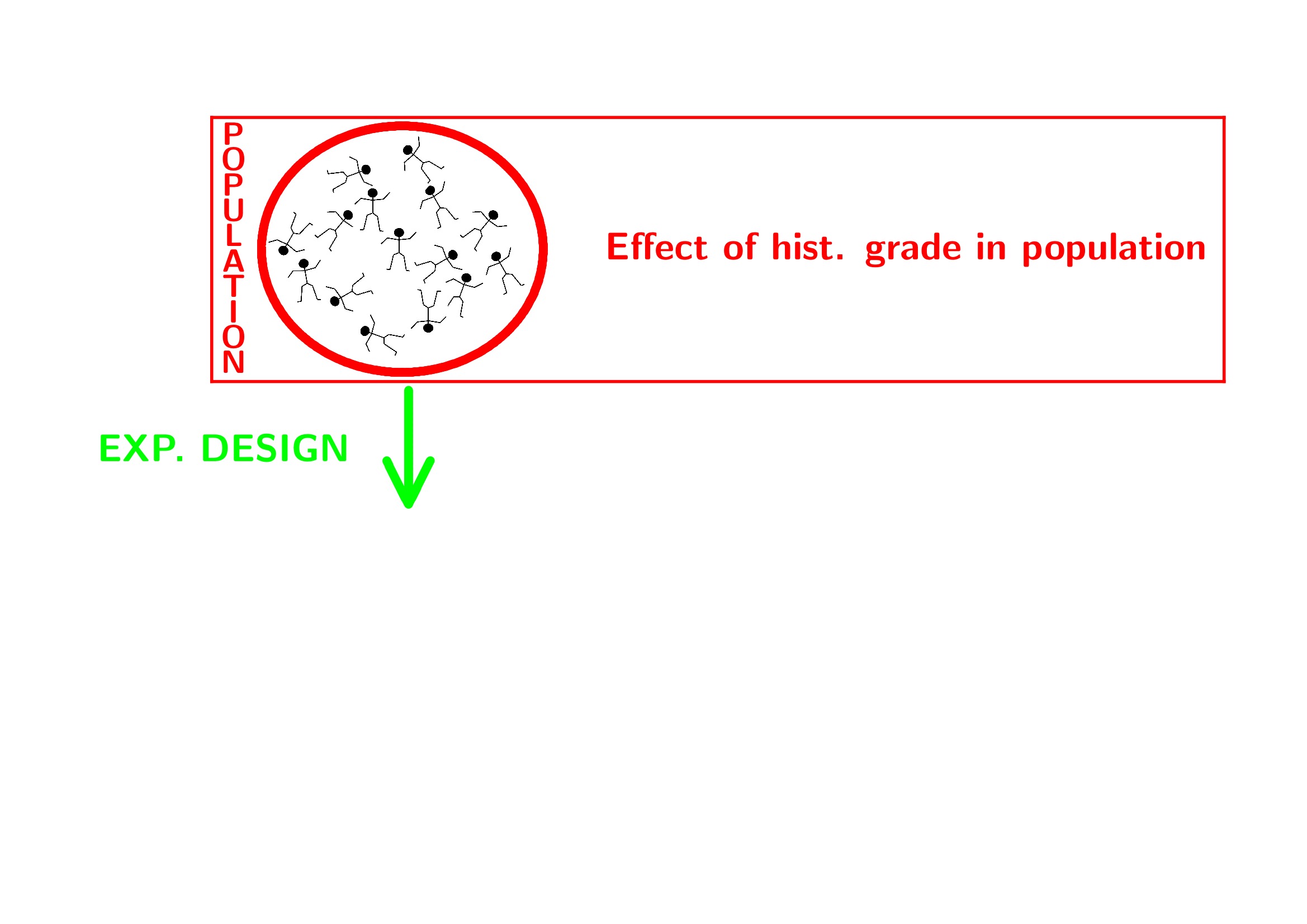
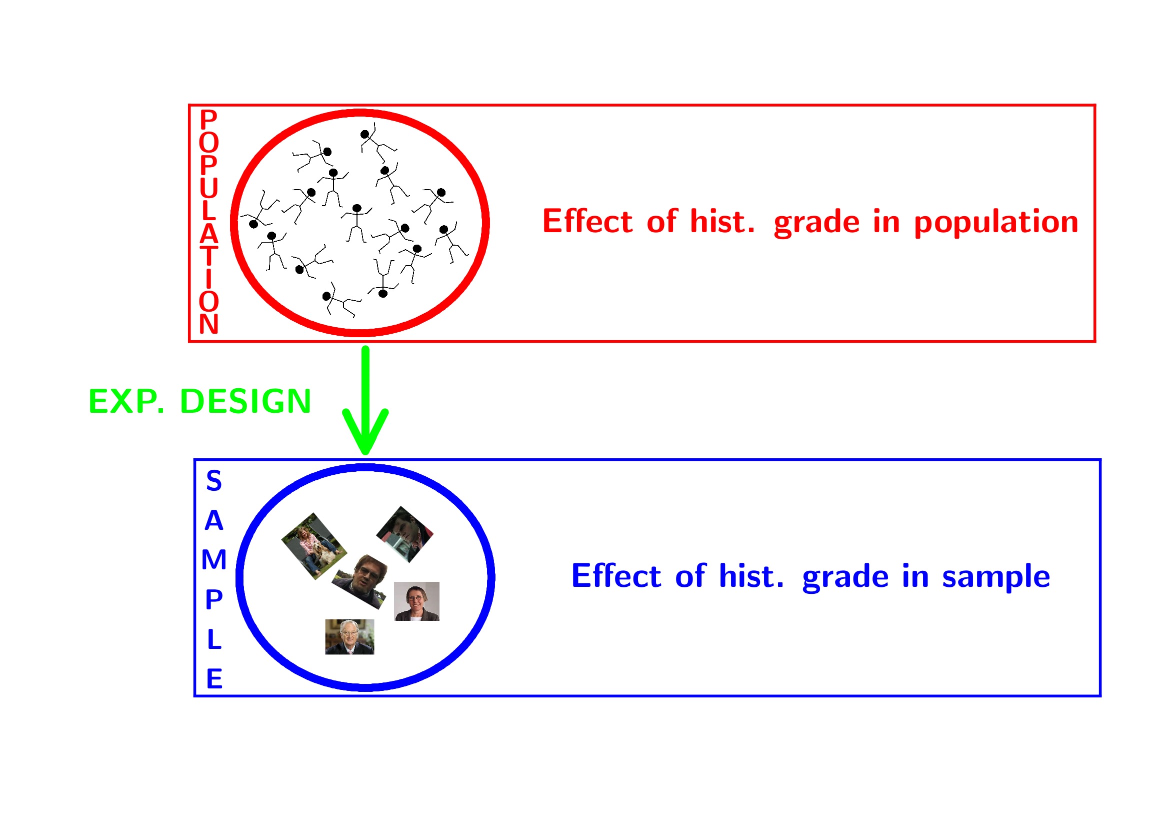
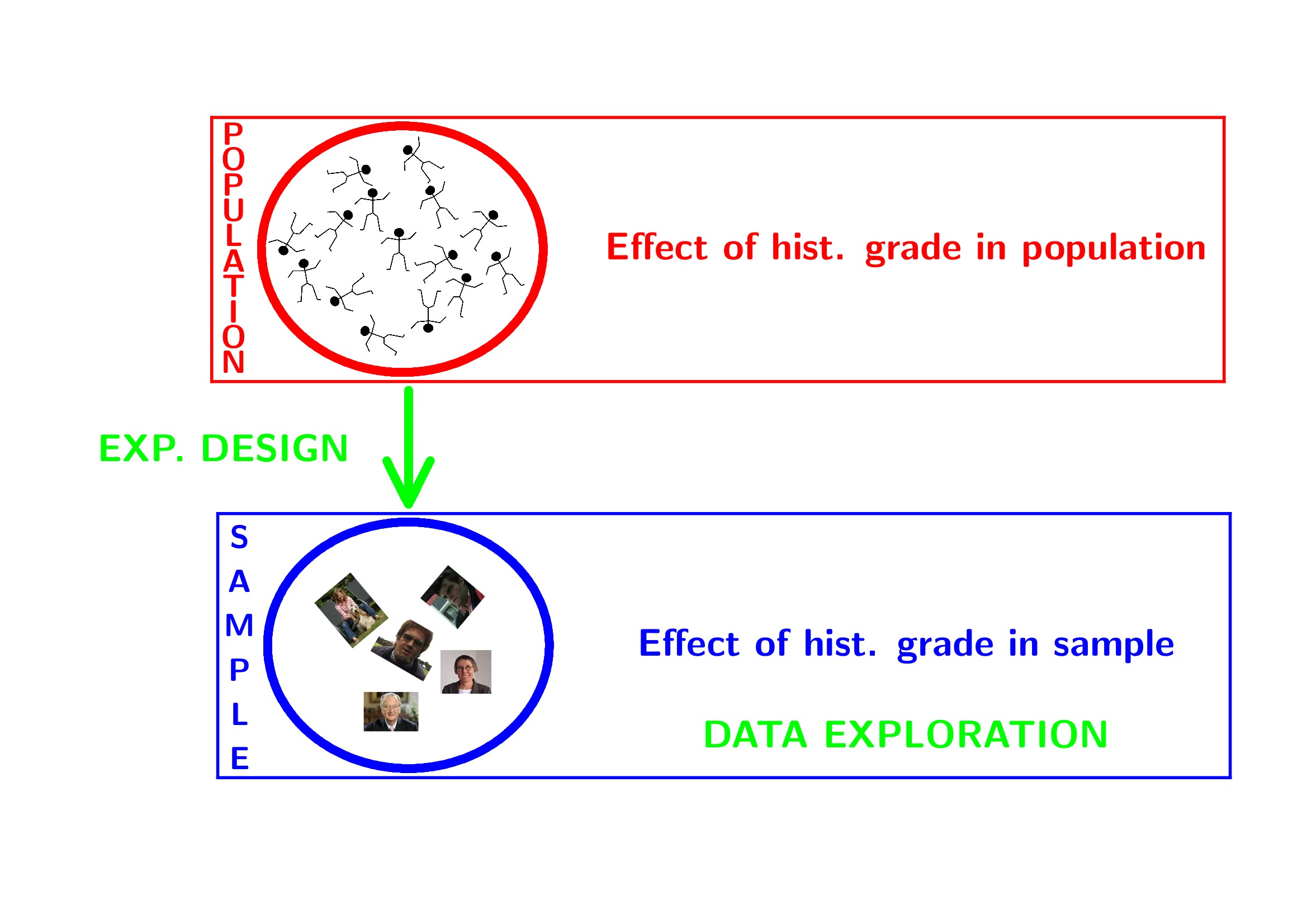
• Population: all current and future breast cancer patients

---

---

---

---

---

---

2 Data Exploration

2.1 Import

library(tidyverse)

## ── Attaching packages ─────────────────────────────────────── tidyverse 1.3.1 ──

## ✔ ggplot2 3.3.5     ✔ purrr   0.3.4
## ✔ tibble  3.1.6     ✔ dplyr   1.0.7
## ✔ tidyr   1.1.4     ✔ stringr 1.4.0
## ✔ readr   2.1.1     ✔ forcats 0.5.1

## ── Conflicts ────────────────────────────────────────── tidyverse_conflicts() ──
## ✖ dplyr::filter() masks stats::filter()
## ✖ dplyr::lag()    masks stats::lag()

gene <- read.table("https://raw.githubusercontent.com/statOmics/SGA21/master/data/kpna2.txt",header=TRUE)
head(gene)

We will transform the variable grade and node to a factor

gene$grade <- as.factor(gene$grade)
gene$node <- as.factor(gene$node)

2.2 Summary statistics

geneSum <- gene %>%
  group_by(grade) %>%
  summarize(mean = mean(gene),
            sd = sd(gene),
            n=length(gene)
            ) %>%
  mutate(se = sd/sqrt(n))
geneSum

2.3 Visualisation

gene %>%
  ggplot(aes(x=grade,y=gene)) +
  geom_boxplot(outlier.shape=NA) +
  geom_jitter()

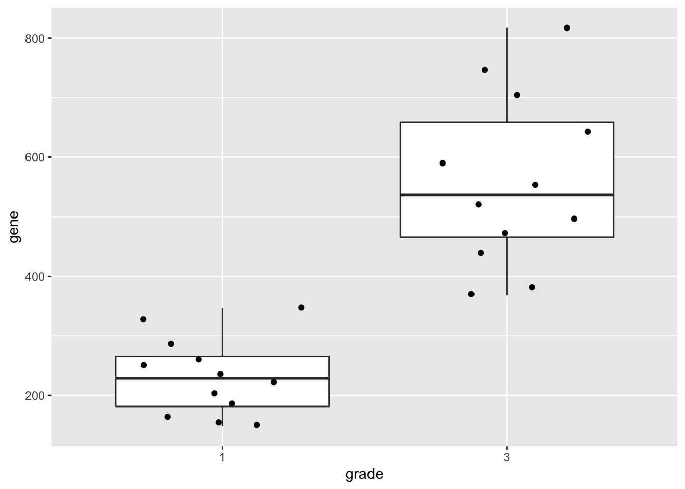
We can also save the plots as objects for later use!

p1 <- gene %>%
  ggplot(aes(x=grade,y=gene)) +
  geom_boxplot(outlier.shape=NA) +
  geom_jitter()

p2 <- gene %>%
  ggplot(aes(sample=gene)) +
  geom_qq() +
  geom_qq_line() +
  facet_wrap(~grade)

p1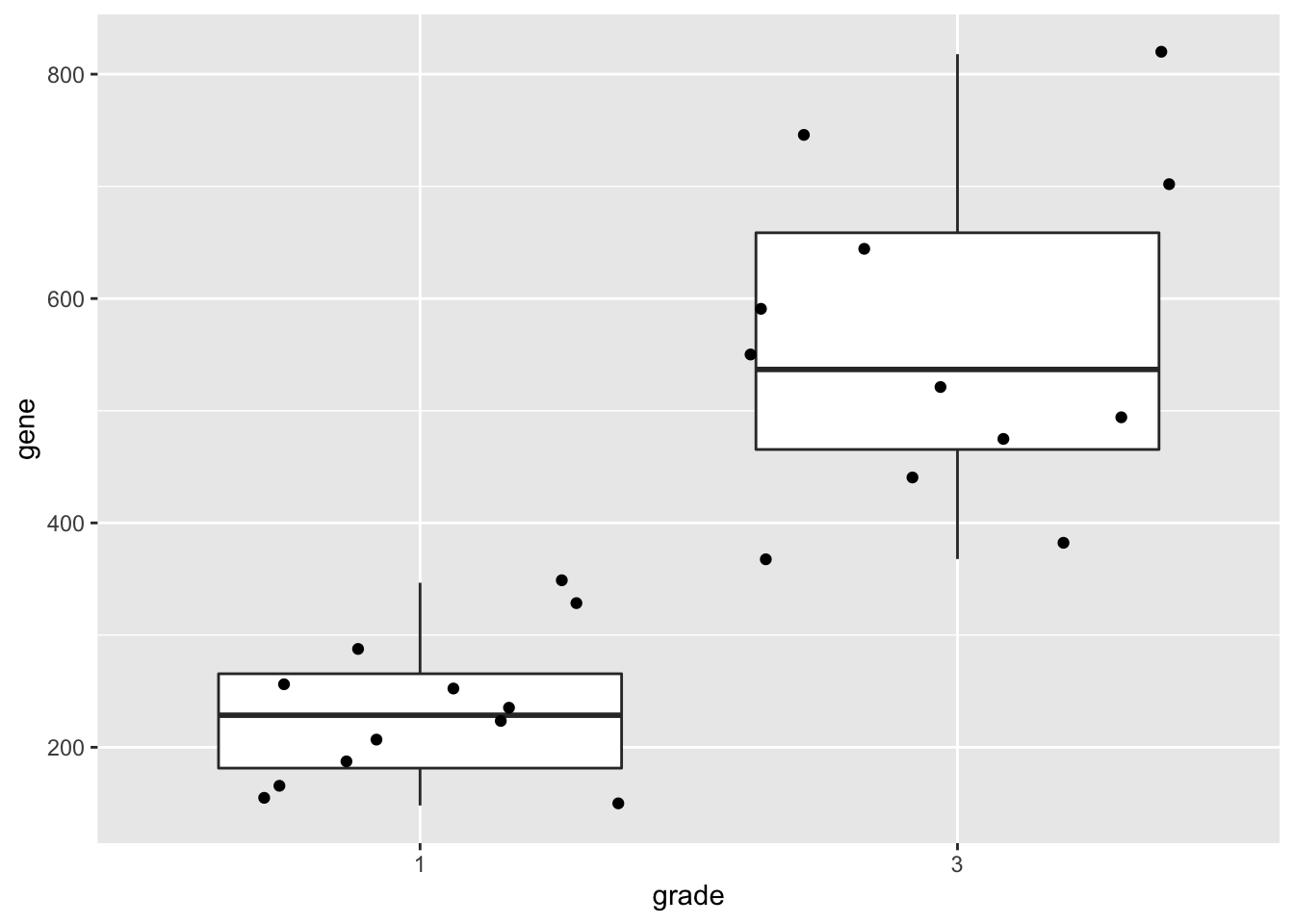

p2

2.4 Research questions

Researchers want to assess the association of the histological grade on KPNA2 gene expression

---

2.5 Estimation of effect size and standard error

effectSize <- tibble(
  delta = geneSum$mean[2]- geneSum$mean[1],
  seDelta = geneSum %>%
    pull(se) %>%
    .^2 %>%
    sum %>%
    sqrt
  )
effectSize

3 Statistical Inference

• Researchers want to assess the association of histological grade on KPNA2 gene expression
• Inference?

---

---

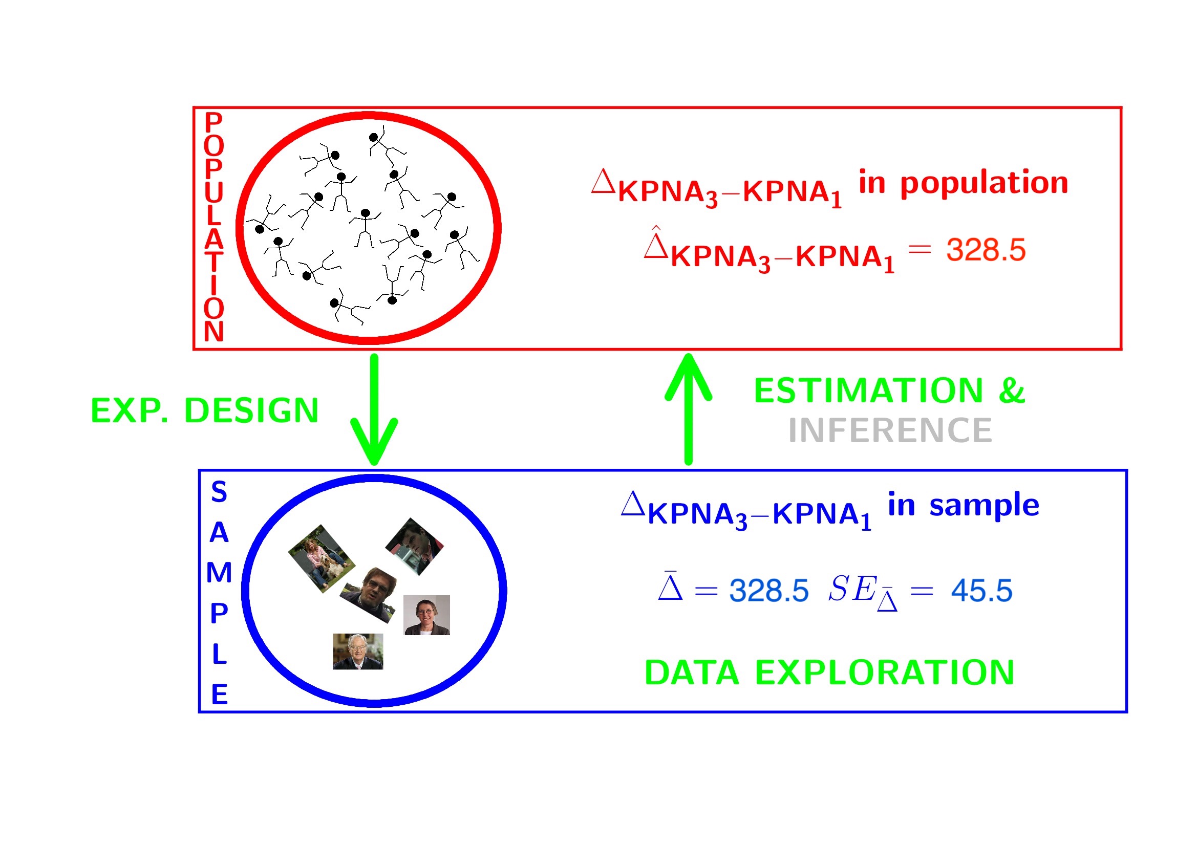
• Researchers want to assess the association of histological grade on KPNA2 gene expression
• Inference?
• testing + CI $ $ Assumptions

---

• In general we start from alternative hypothese \(H_A\): we want to show an association

• Gene expression of grade 1 and grade 3 patients is on average different

• But, we will assess it by falsifying the opposite:

• The average KPNA2 gene expression of grade 1 and grade 3 patients is equal

---

• How likely is it to observe an equal or more extreme association than the one observed in the sample when the null hypothesis is true?

• When we make assumptions about the distribution of our test statistic we can quantify this probability: p-value.

• If the p-value is below a significance threshold \(\alpha\) we reject the null hypothesis

We control the probability on a false positive result at the \(\alpha\)-level (type I error)

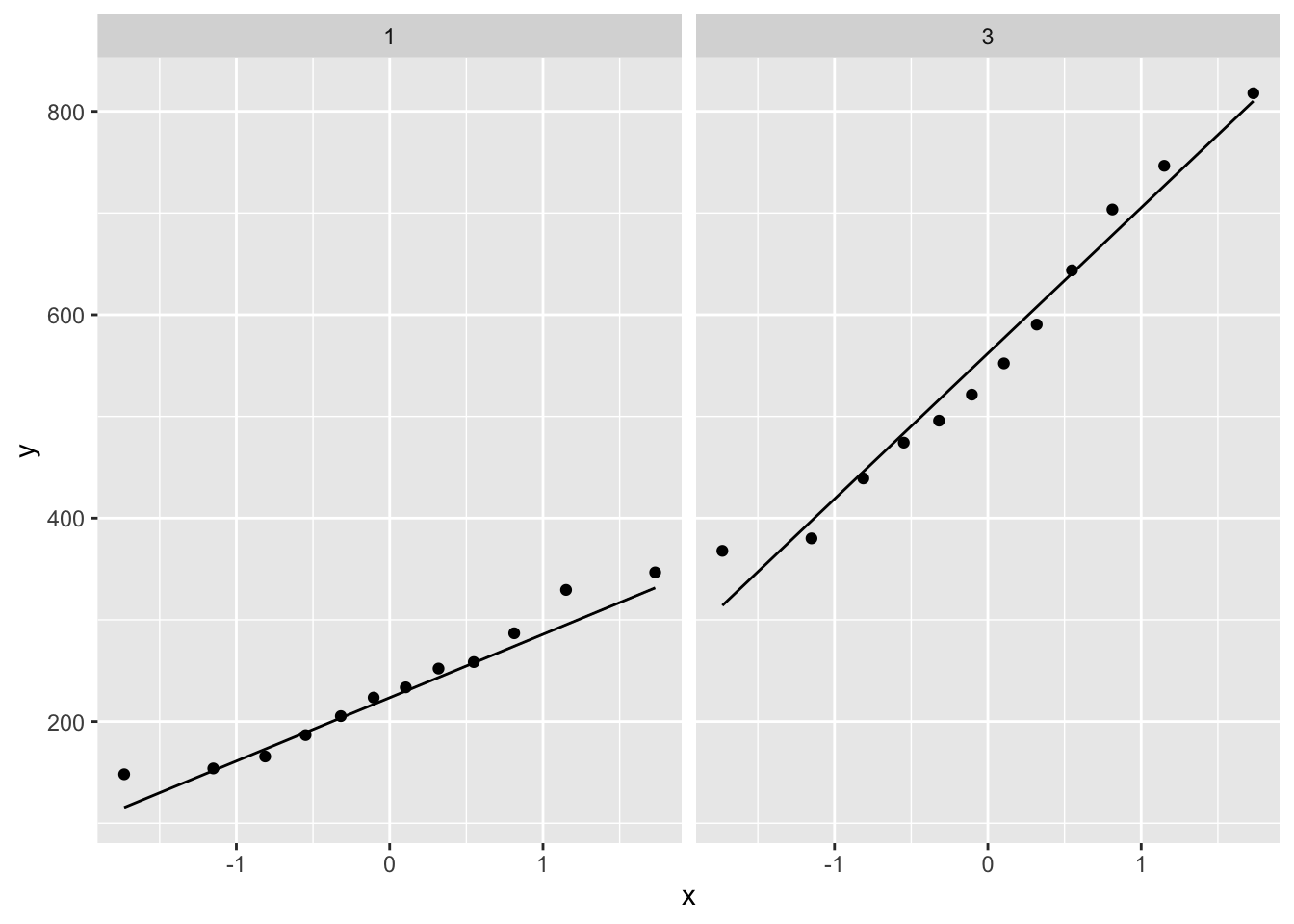
• The p-value will only be calculated correctly if the underlying assumptions hold!

library(gridExtra)

## 
## Attaching package: 'gridExtra'

## The following object is masked from 'package:dplyr':
## 
##     combine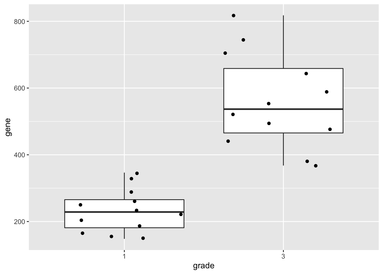

p1

p2

t.test(gene~grade,data=gene)

## 
##  Welch Two Sample t-test
## 
## data:  gene by grade
## t = -7.2132, df = 15.384, p-value = 2.598e-06
## alternative hypothesis: true difference in means between group 1 and group 3 is not equal to 0
## 95 percent confidence interval:
##  -425.4218 -231.6751
## sample estimates:
## mean in group 1 mean in group 3 
##        232.5003        561.0487

effectSize <- effectSize %>%
  mutate(t.stat=delta/seDelta) %>%
  mutate(p.value= pt(-abs(t.stat),21.352)*2)

effectSize

• Intensities are often not normally distributed and have a mean variance relation
• Commonly log2-transformed
• Differences on log scale:

\[ \log_2(B) - \log_2(A) = \log_2 \frac{B}{A} = \log_2 FC_{\frac{B}{A}} \]

---

3.1 Log transformation

gene <- gene %>%
  mutate(lgene = log2(gene))

p1 <- gene %>%
  ggplot(aes(x=grade,y=lgene)) +
  geom_boxplot(outlier.shape=NA) +
  geom_jitter()

p2 <- gene %>%
  ggplot(aes(sample=lgene)) +
  geom_qq() +
  geom_qq_line() +
  facet_wrap(~grade)

p1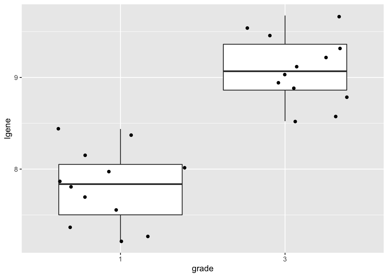

p2

logtest <- t.test(lgene~grade,data=gene,var.equal=TRUE)
logtest

## 
##  Two Sample t-test
## 
## data:  lgene by grade
## t = -8.0455, df = 22, p-value = 5.372e-08
## alternative hypothesis: true difference in means between group 1 and group 3 is not equal to 0
## 95 percent confidence interval:
##  -1.610148 -0.950178
## sample estimates:
## mean in group 1 mean in group 3 
##        7.808478        9.088641

log2FC <- logtest$estimate[2]-logtest$estimate[1]
log2FC

## mean in group 3 
##        1.280163

names(log2FC) <- "g3-g1"
2^log2FC

##    g3-g1 
## 2.428664

3.2 Conclusion

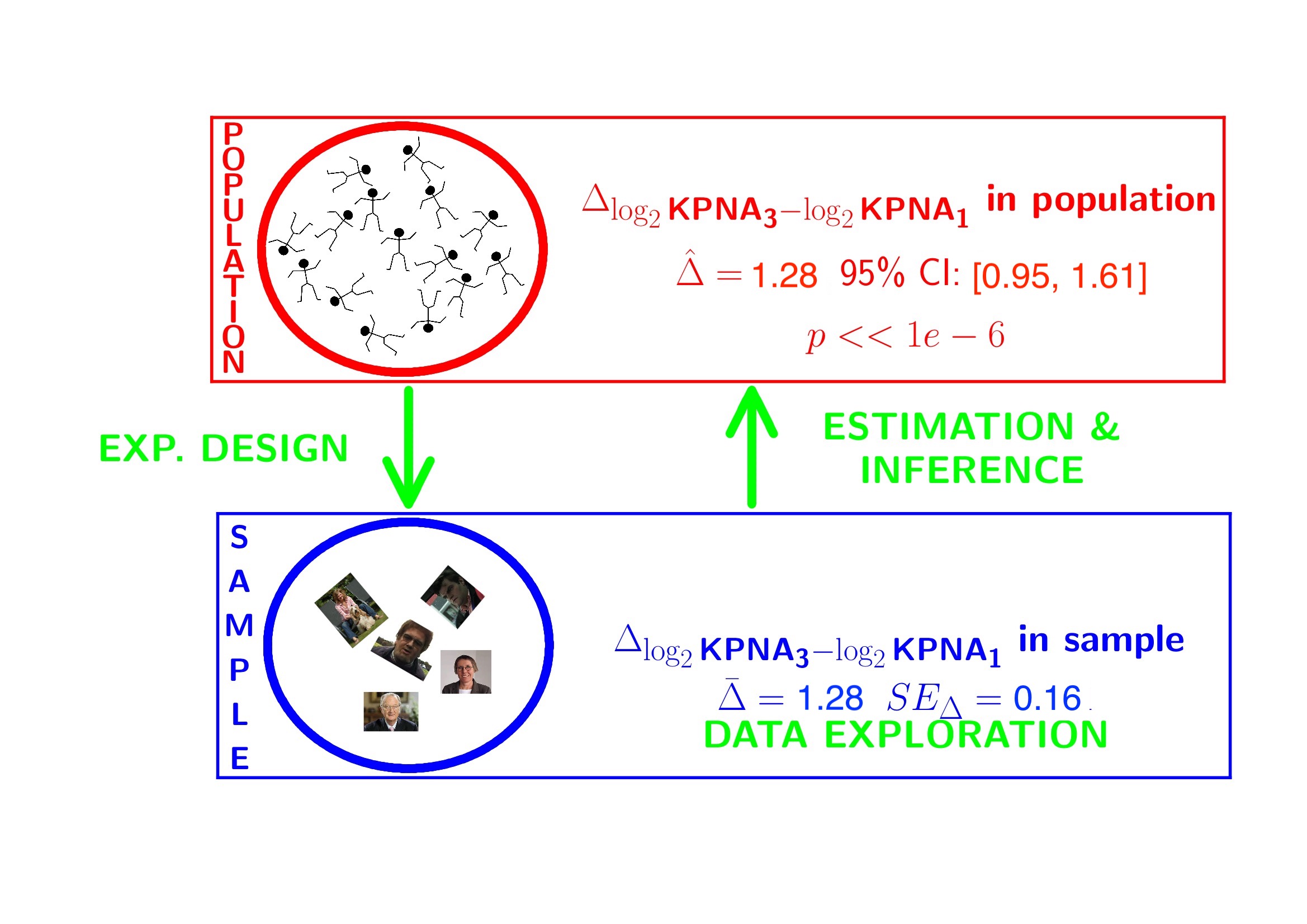
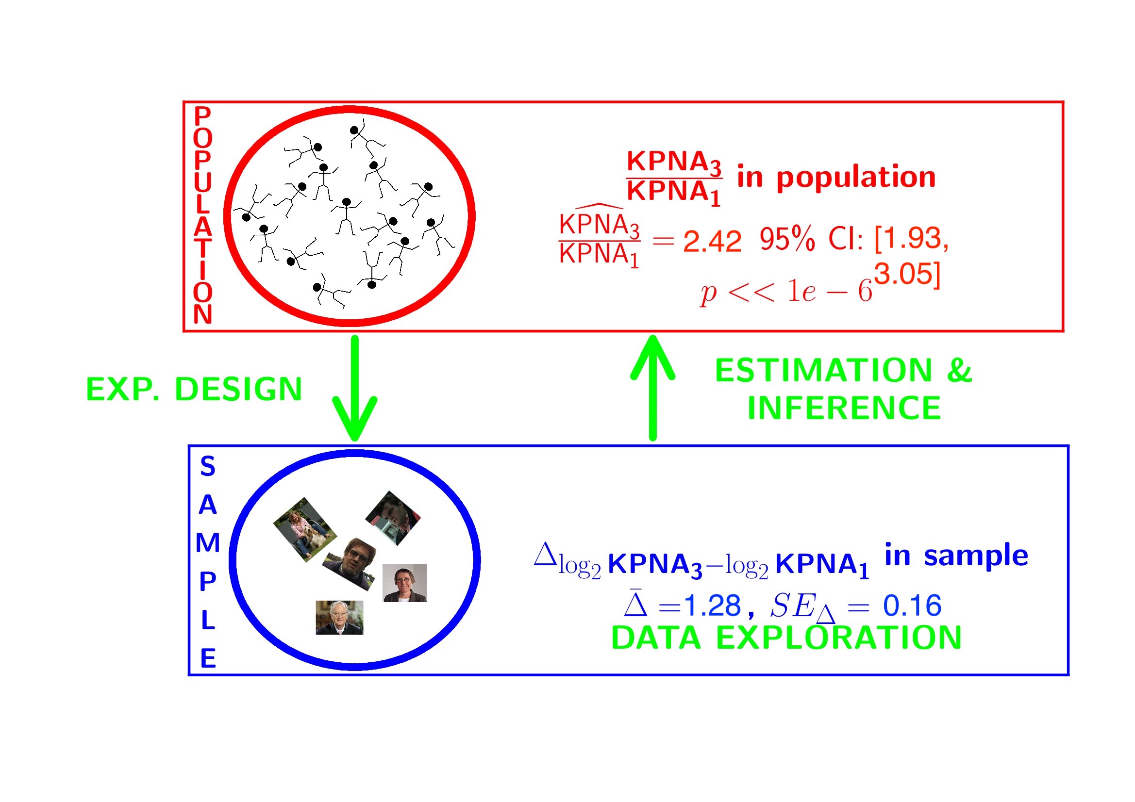
There is a extremely significant association of the histological grade on the gene expression in tumor tissue. On average, the gene expression for the grade 3 patients is 2.43 times higher than the gene expression in grade 1 patients (95% CI [1.93, 3.05], \(p<<0.001\)).

---

---

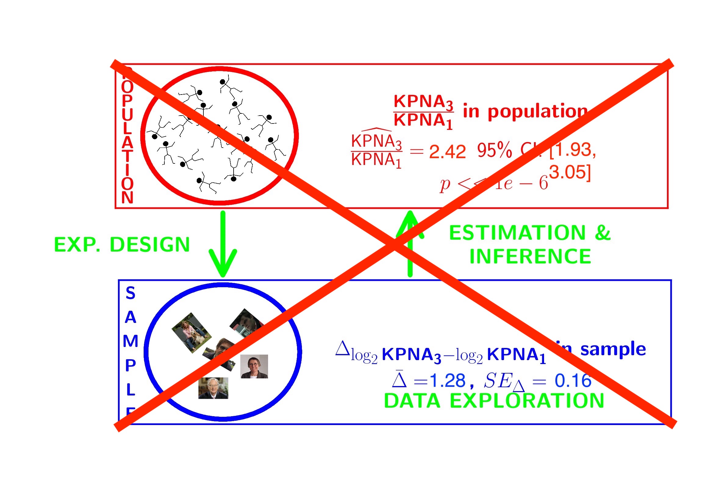
The patients also differ in the their lymph node status. Hence, we have a two factorial design: grade x lymph node status!!!

Solution??

---

4 General Linear Model

How can we integrate multiple factors and continuous covariates in linear model.

\[ y_i= \beta_0 + \beta_1 x_{i,1} + \beta_2 x_{i,2} + \beta_{12}x_{i,1}x_{i,2}+\epsilon_i, \] with

• \(x_{i,1}\) a dummy variable for histological grade: \(x_{i,1}=\begin{cases} 0& \text{grade 1}\\ 1& \text{grade 3} \end{cases}\)
• \(x_{i,2}\) a dummy variable for : \(x_{i,2}=\begin{cases} 0& \text{lymph nodes were not removed}\\ 1& \text{lymph nodes were removed} \end{cases}\)
• \(\epsilon_i\)?

---

4.1 Implementation in R

lm1 <- lm(gene~grade*node,data=gene)
summary(lm1)

## 
## Call:
## lm(formula = gene ~ grade * node, data = gene)
## 
## Residuals:
##      Min       1Q   Median       3Q      Max 
## -201.748  -53.294   -6.308   46.216  277.601 
## 
## Coefficients:
##              Estimate Std. Error t value Pr(>|t|)    
## (Intercept)    180.51      44.37   4.068   0.0006 ***
## grade3         401.33      62.75   6.396 3.07e-06 ***
## node1          103.98      62.75   1.657   0.1131    
## grade3:node1  -145.57      88.74  -1.640   0.1166    
## ---
## Signif. codes:  0 '***' 0.001 '**' 0.01 '*' 0.05 '.' 0.1 ' ' 1
## 
## Residual standard error: 108.7 on 20 degrees of freedom
## Multiple R-squared:  0.7437, Adjusted R-squared:  0.7052 
## F-statistic: 19.34 on 3 and 20 DF,  p-value: 3.971e-06

---

4.2 Assumptions

plot(lm1)

---

4.3 Breast cancer example

• Paper: https://doi.org/10.1093/jnci/djj052
• Histologic grade in breast cancer provides clinically important prognostic information. Two factors have to be concidered: Histologic grade (grade 1 and grade 3) and lymph node status (0 vs 1). The researchers assessed gene expression of the KPNA2 gene a protein-coding gene associated with breast cancer and are mainly interested in the association of histological grade. Note, that the gene variable consists of background corrected normalized intensities obtained with a microarray platform. Upon log-transformation, they are known to be a good proxy for the \(\log\) transformed concentration of gene expression product of the KPNA2 gene.
• Research questions and translate them towards model parameters (contrasts)?
• Make an R markdown file to answer the research questions

library(ExploreModelMatrix)
explMx <- VisualizeDesign(gene,designFormula = ~grade*node)
explMx$plotlist

## [[1]]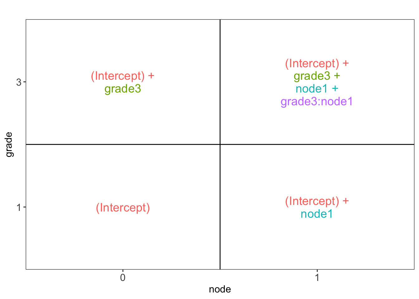

You can also explore the model matrix interactively:

ExploreModelMatrix(gene,designFormula = ~grade*node)

---

5 Linear regression in matrix form

5.1 Scalar form

• Consider a vector of predictors \(\mathbf{x}=(x_1,\ldots,x_p)^T\) and
• a real-valued response \(Y\)
• then the linear regression model can be written as \[ Y=f(\mathbf{x}) +\epsilon=\beta_0+\sum\limits_{j=1}^p x_j\beta_j + \epsilon \] with i.i.d. \(\epsilon\sim N(0,\sigma^2)\)

5.2 Matrix form

• \(n\) observations \((\mathbf{x}_1,y_1) \ldots (\mathbf{x}_n,y_n)\)
• Regression in matrix notation \[\mathbf{Y}=\mathbf{X\beta} + \mathbf{\epsilon}\] with \(\mathbf{Y}=\left[\begin{array}{c}y_1\\ \vdots\\y_n\end{array}\right]\), \(\mathbf{X}=\left[\begin{array}{cccc} 1&x_{11}&\ldots&x_{1p}\\ \vdots&\vdots&&\vdots\\ 1&x_{n1}&\ldots&x_{np} \end{array}\right]\), \(\mathbf{\beta}=\left[\begin{array}{c}\beta_0\\ \vdots\\ \beta_p\end{array}\right]\) and \(\mathbf{\epsilon}=\left[\begin{array}{c} \epsilon_1 \\ \vdots \\ \epsilon_n\end{array}\right]\)

5.3 Least Squares (LS)

• Minimize the residual sum of squares \[\begin{eqnarray*} RSS(\mathbf{\beta})&=&\sum\limits_{i=1}^n e^2_i\\ &=&\sum\limits_{i=1}^n \left(y_i-\beta_0-\sum\limits_{j=1}^p x_{ij}\beta_j\right)^2 \end{eqnarray*}\]
• or in matrix notation \[\begin{eqnarray*} RSS(\mathbf{\beta})&=&(\mathbf{Y}-\mathbf{X\beta})^T(\mathbf{Y}-\mathbf{X\beta})\\ &=&\Vert \mathbf{Y}-\mathbf{X\beta}\Vert^2_2 \end{eqnarray*}\] with the \(L_2\)-norm of a \(p\)-dim. vector \(v\) \(\Vert \mathbf{v} \Vert=\sqrt{v_1^2+\ldots+v_p^2}\) \(\rightarrow\) \(\hat{\mathbf{\beta}}=\text{argmin}_\beta \Vert \mathbf{Y}-\mathbf{X\beta}\Vert^2_2\)

---

5.3.1 Minimize RSS

\[ \begin{array}{ccc} \frac{\partial RSS}{\partial \mathbf{\beta}}&=&\mathbf{0}\\\\ \frac{(\mathbf{Y}-\mathbf{X\beta})^T(\mathbf{Y}-\mathbf{X\beta})}{\partial \mathbf{\beta}}&=&\mathbf{0}\\\\ -2\mathbf{X}^T(\mathbf{Y}-\mathbf{X\beta})&=&\mathbf{0}\\\\ \mathbf{X}^T\mathbf{X\beta}&=&\mathbf{X}^T\mathbf{Y}\\\\ \hat{\mathbf{\beta}}&=&(\mathbf{X}^T\mathbf{X})^{-1}\mathbf{X}^T\mathbf{Y} \end{array} \]

---

5.3.2 Geometrical Interpretation

Toy Example: fit without intercept

• n=3 and p=2 \[ \mathbf{X}=\left[\begin{array}{cc} 2&0\\ 0&2\\ 0&0 \end{array}\right] \]

set.seed(4)
x1 <- c(2,0,0)
x2 <- c(0,2,0)
y <- x1*0.5 + x2*0.5 + rnorm(3,2)
fit <- lm(y~-1+x1+x2)

5.3.2.1 Visualise fit

# predict values on regular xy grid
x1pred <- seq(-1, 3, length.out = 10)
x2pred <- seq(-1, 3, length.out = 10)
xy <- expand.grid(x1 = x1pred,
x2 = x2pred)
ypred <- matrix (nrow = 30, ncol = 30,
data = predict(fit, newdata = data.frame(xy),
interval = "prediction"))

library(plot3D)

## Warning in fun(libname, pkgname): no display name and no $DISPLAY environment
## variable

# fitted points for droplines to surface
th=20
ph=5
scatter3D(x1,
  x2,
  y,
  pch = 16,
  col="darkblue",
  cex = 1,
  theta = th,
  ticktype = "detailed",
  xlab = "x1",
  ylab = "x2",
  zlab = "y",  
  colvar=FALSE,
  bty = "g",
  xlim=c(-1,3),
  ylim=c(-1,3),
  zlim=c(-2,4))

for (i in 1:3)
  lines3D(
    x = rep(x1[i],2),
    y = rep(x2[i],2),
    z = c(y[i],fit$fitted[i]),
    col="darkblue",
    add=TRUE,
    lty=2)

z.pred3D <- outer(
  x1pred,
  x2pred,
  function(x1,x2)
  {
    fit$coef[1]*x1+fit$coef[2]*x2
  })

x.pred3D <- outer(
  x1pred,
  x2pred,
  function(x,y) x)

y.pred3D <- outer(
  x1pred,
  x2pred,
  function(x,y) y)

surf3D(
  x.pred3D,
  y.pred3D,
  z.pred3D,
  col="blue",
  facets=NA,
  add=TRUE)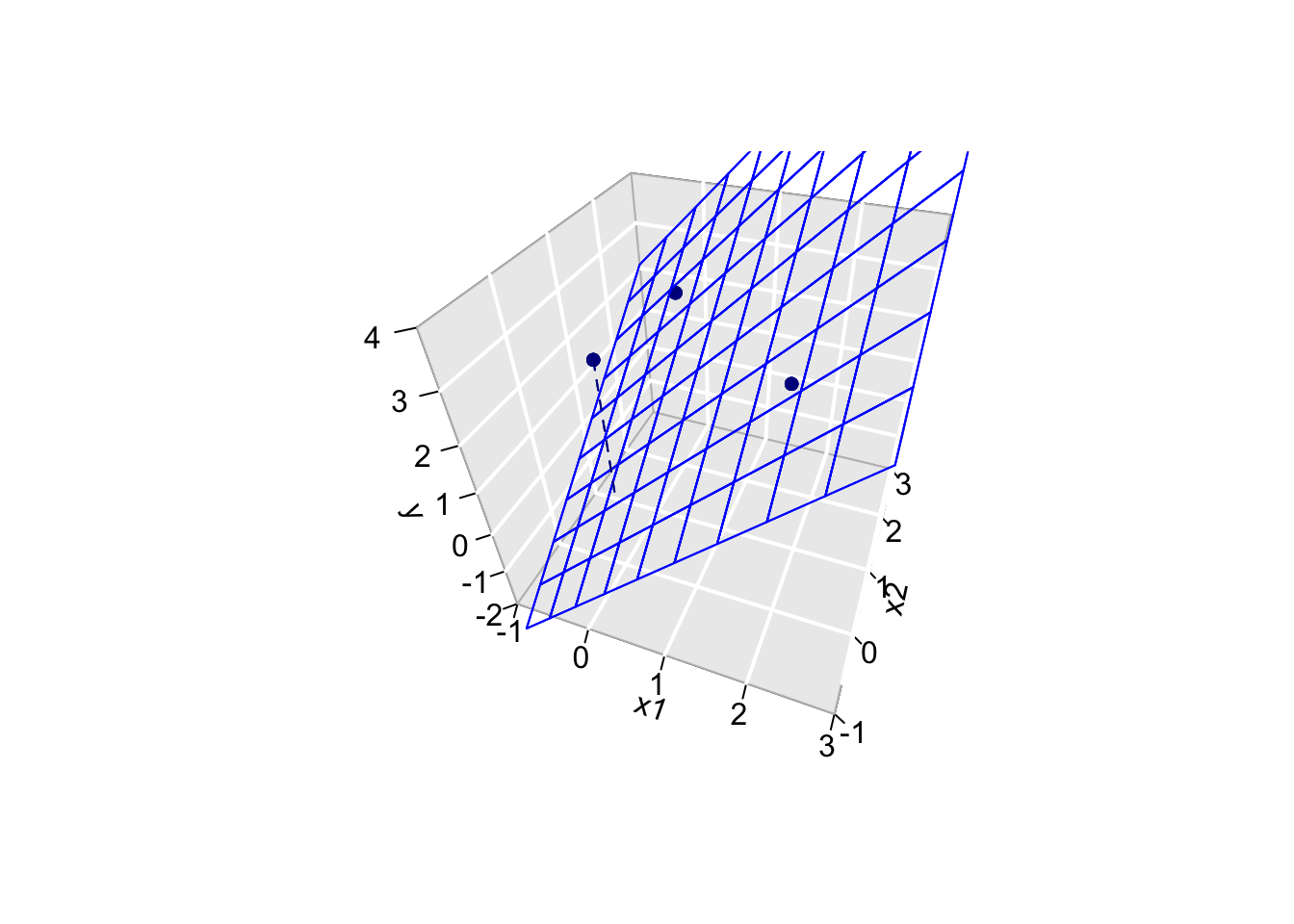

5.3.3 Projection

• We can also interpret the fit as the projection of the \(n\times 1\) vector \(\mathbf{Y}\) on the column space of the matrix \(\mathbf{X}\).

• So each column in \(\mathbf{X}\) is also an \(n\times 1\) vector.

• For the toy example n=3 and p=2. So the column space of X is a plane in the three dimensional space.

\[ \hat{\mathbf{Y}} = \mathbf{X} (\mathbf{X}^T\mathbf{X})^{-1} \mathbf{X}^T \mathbf{Y} \]

1. Plane spanned by column space:

arrows3D(0,0,0,x1[1],x1[2],x1[3],xlim=c(0,5),ylim=c(0,5),zlim=c(0,5),bty = "g",theta=th,col=2,xlab="row 1",ylab="row 2",zlab="row 3")
text3D(x1[1],x1[2],x1[3],labels="X1",col=2,add=TRUE)
arrows3D(0,0,0,x2[1],x2[2],x2[3],add=TRUE,col=2)
text3D(x2[1],x2[2],x2[3],labels="X2",col=2,add=TRUE)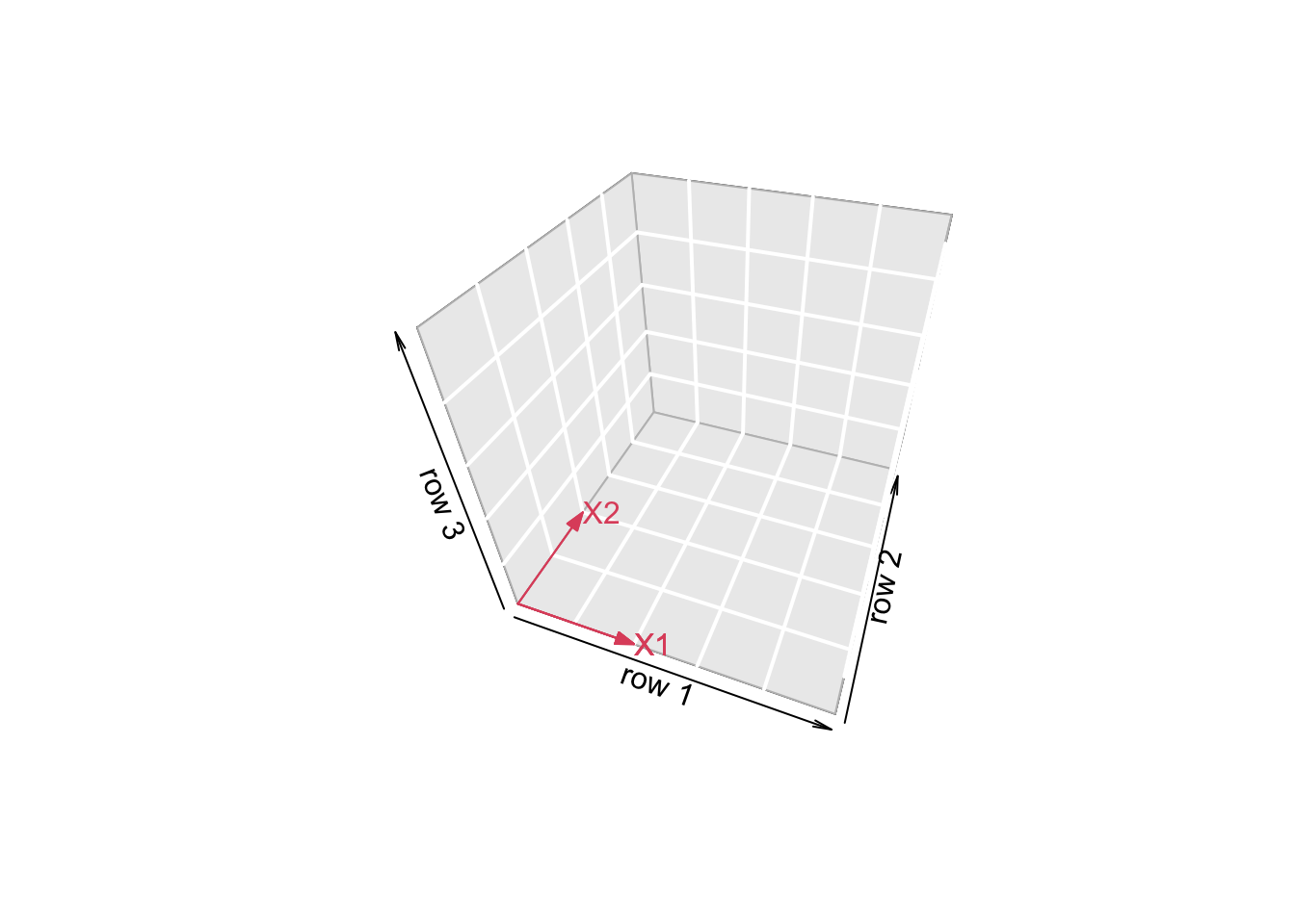

2. Vector of Y:

arrows3D(0,0,0,x1[1],x1[2],x1[3],xlim=c(0,5),ylim=c(0,5),zlim=c(0,5),bty = "g",theta=th,col=2,xlab="row 1",ylab="row 2",zlab="row 3")
text3D(x1[1],x1[2],x1[3],labels="X1",col=2,add=TRUE)
arrows3D(0,0,0,x2[1],x2[2],x2[3],add=TRUE,col=2)
text3D(x2[1],x2[2],x2[3],labels="X2",col=2,add=TRUE)
arrows3D(0,0,0,y[1],y[2],y[3],add=TRUE,col="darkblue")
text3D(y[1],y[2],y[3],labels="Y",col="darkblue",add=TRUE)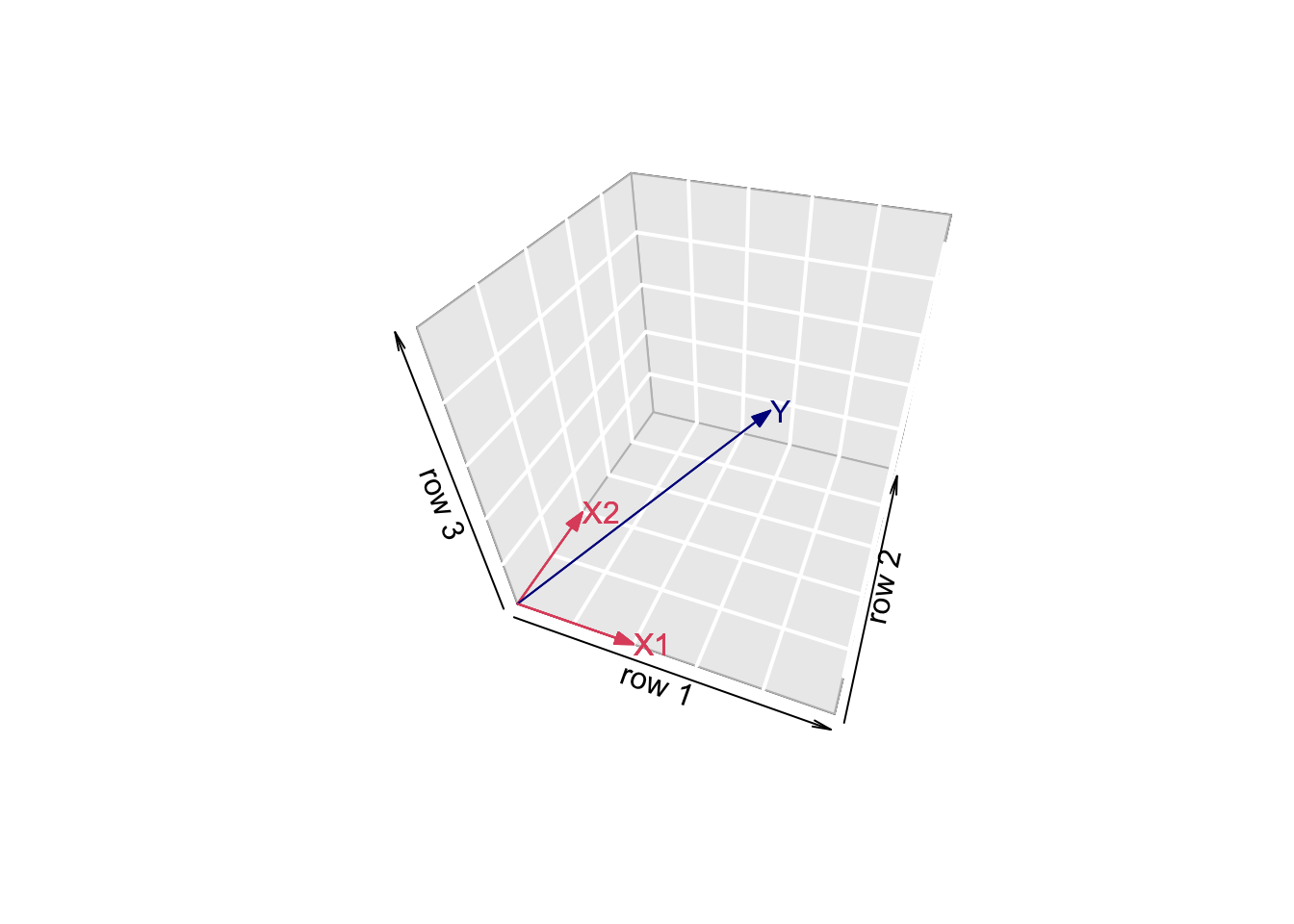

3. Projection of Y onto column space

arrows3D(0,0,0,x1[1],x1[2],x1[3],xlim=c(0,5),ylim=c(0,5),zlim=c(0,5),bty = "g",theta=th,col=2,xlab="row 1",ylab="row 2",zlab="row 3")
text3D(x1[1],x1[2],x1[3],labels="X1",col=2,add=TRUE)
arrows3D(0,0,0,x2[1],x2[2],x2[3],add=TRUE,col=2)
text3D(x2[1],x2[2],x2[3],labels="X2",col=2,add=TRUE)
arrows3D(0,0,0,y[1],y[2],y[3],add=TRUE,col="darkblue")
text3D(y[1],y[2],y[3],labels="Y",col="darkblue",add=TRUE)
arrows3D(0,0,0,fit$fitted[1],fit$fitted[2],fit$fitted[3],add=TRUE,col="darkblue")
segments3D(y[1],y[2],y[3],fit$fitted[1],fit$fitted[2],fit$fitted[3],add=TRUE,lty=2,col="darkblue")
text3D(fit$fitted[1],fit$fitted[2],fit$fitted[3],labels="fit",col="darkblue",add=TRUE)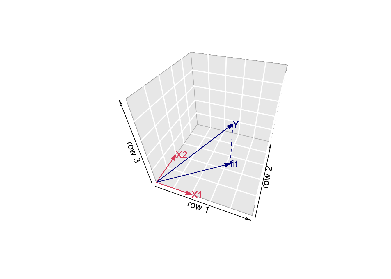

• Note, that it is also clear from the equation in the derivation of the LS that the residual is orthogonal on the column space: \[ -2 \mathbf{X}^T(\mathbf{Y}-\mathbf{X}\boldsymbol{\beta}) = 0 \]

---

5.4 Variance Estimator?

\[ \begin{array}{ccl} \hat{\boldsymbol{\Sigma}}_{\hat{\mathbf{\beta}}} &=&\text{var}\left[(\mathbf{X}^T\mathbf{X})^{-1}\mathbf{X}^T\mathbf{Y}\right]\\\\ &=&(\mathbf{X}^T\mathbf{X})^{-1}\mathbf{X}^T\text{var}\left[\mathbf{Y}\right]\mathbf{X}(\mathbf{X}^T\mathbf{X})^{-1}\\\\ &=&(\mathbf{X}^T\mathbf{X})^{-1}\mathbf{X}^T(\mathbf{I}\sigma^2)\mathbf{X}(\mathbf{X}^T\mathbf{X})^{-1} \\\\ &=&(\mathbf{X}^T\mathbf{X})^{-1}\mathbf{X}^T\mathbf{I}\quad\mathbf{X}(\mathbf{X}^T\mathbf{X})^{-1}\sigma^2\\\\ %\hat{\boldmath{\Sigma}}_{\hat{\mathbf{\beta}}}&=&(\mathbf{X}^T\mathbf{X})^{-1}\mathbf{X}^T\var\left[\mathbf{Y}\right](\mathbf{X}^T\mathbf{X})^{-1}\mathbf{X}\\ &=&(\mathbf{X}^T\mathbf{X})^{-1}\mathbf{X}^T\mathbf{X}(\mathbf{X}^T\mathbf{X})^{-1}\sigma^2\\\\ &=&(\mathbf{X}^T\mathbf{X})^{-1}\sigma^2 \end{array} \]

---

5.5 Contrasts

Hypotheses often involve linear combinations of the model parameters!

e.g.

• \(H_0: \log_2{FC}_{g3n1-g1n1}= \beta_{g3} + \hat\beta_{g3n1}=0\) \(\rightarrow\) “grade3+grade3:node1 = 0”

• Let \[ \boldsymbol{\beta} = \left[ \begin{array}{c} \beta_{0}\\ \beta_{g3}\\ \beta_{n1}\\ \beta_{g3:n1} \end{array} \right]\]

• we can write that contrast using a contrast matrix: \[ \mathbf{L}=\left[\begin{array}{c}0\\1\\0\\1\end{array}\right] \rightarrow \mathbf{L}^T\boldsymbol{beta} \]

• Then the variance becomes: \[ \text{var}_{\mathbf{L}^T\boldsymbol{\hat\beta}}= \mathbf{L}^T \boldsymbol{\Sigma}_{\boldsymbol{\hat\beta}}\mathbf{L} \]

---

6 Homework: Adopt the gene analysis on log scale in matrix form!

1. Study the solution of the exercise to understand the analysis in R

2. Calculate

• model parameters and contrasts of interest
• standard errors, standard errors on contrasts
• t-test statistics on the model parameters and contrasts of interest

3. Compare your results with the output of the lm(.) function

---

6.1 Inspiration

Tip: details on the implementation can be found in the book of Faraway (chapter 2). https://people.bath.ac.uk/jjf23/book/

• Design matrix

X <- model.matrix(~grade*node,data=gene)

• Transpose of a matrix: use function t(.)

t(X)

##              1 2 3 4 5 6 7 8 9 10 11 12 13 14 15 16 17 18 19 20 21 22 23 24
## (Intercept)  1 1 1 1 1 1 1 1 1  1  1  1  1  1  1  1  1  1  1  1  1  1  1  1
## grade3       1 1 0 0 0 1 1 0 1  1  0  1  0  0  0  1  0  1  0  1  0  1  1  0
## node1        1 1 1 1 0 0 1 1 0  0  0  0  0  0  0  1  1  0  1  1  1  0  1  0
## grade3:node1 1 1 0 0 0 0 1 0 0  0  0  0  0  0  0  1  0  0  0  1  0  0  1  0
## attr(,"assign")
## [1] 0 1 2 3
## attr(,"contrasts")
## attr(,"contrasts")$grade
## [1] "contr.treatment"
## 
## attr(,"contrasts")$node
## [1] "contr.treatment"

• Matrix product %*% operator

t(X)%*%X

##              (Intercept) grade3 node1 grade3:node1
## (Intercept)           24     12    12            6
## grade3                12     12     6            6
## node1                 12      6    12            6
## grade3:node1           6      6     6            6

• Degrees of freedom of a model?

\[ df = n-p\]

summary(lm1)

## 
## Call:
## lm(formula = gene ~ grade * node, data = gene)
## 
## Residuals:
##      Min       1Q   Median       3Q      Max 
## -201.748  -53.294   -6.308   46.216  277.601 
## 
## Coefficients:
##              Estimate Std. Error t value Pr(>|t|)    
## (Intercept)    180.51      44.37   4.068   0.0006 ***
## grade3         401.33      62.75   6.396 3.07e-06 ***
## node1          103.98      62.75   1.657   0.1131    
## grade3:node1  -145.57      88.74  -1.640   0.1166    
## ---
## Signif. codes:  0 '***' 0.001 '**' 0.01 '*' 0.05 '.' 0.1 ' ' 1
## 
## Residual standard error: 108.7 on 20 degrees of freedom
## Multiple R-squared:  0.7437, Adjusted R-squared:  0.7052 
## F-statistic: 19.34 on 3 and 20 DF,  p-value: 3.971e-06

dfRes <- (nrow(X)-ncol(X))
dfRes

## [1] 20

• Variance estimator: MSE

\[ \hat \sigma^2 = \frac{\sum\limits_{i=1}^n\epsilon_i^2}{n-p} \]

• Invert matrix: use function solve(.)

• Diagonal elements of a matrix: use function diag(.)

t(X)%*%X

##              (Intercept) grade3 node1 grade3:node1
## (Intercept)           24     12    12            6
## grade3                12     12     6            6
## node1                 12      6    12            6
## grade3:node1           6      6     6            6

diag(t(X)%*%X)

##  (Intercept)       grade3        node1 grade3:node1 
##           24           12           12            6