7  Heart use case: a MaxQuant LFQ DDA dataset with a more complex design

7.1 Introduction

In this chapter we show how to analyse LFQ data from an experiment with a more complex design. The data are a small subset of the public dataset PXD006675 on PRIDE.

Particularly, the proteomes of the atrium and ventriculum in the left and the right heart region are profiled for 3 patients (identifiers 3, 4, and 8). Hence, the design consists of a factor tissue (atrium, ventriculum), region (left, right) and block (patient 3,4, and 8).

Suppose that researchers are mainly interested in comparing the ventricular to the atrial proteome. Particularly, they would like to compare the left atrium to the left ventricle, the right atrium to the right ventricle, the average ventricular vs atrial proteome and if ventricular vs atrial proteome shifts differ between left and right heart region.

7.2 Load packages

First, we load the msqrob2 package and additional packages for data manipulation and visualisation.

suppressPackageStartupMessages({
library("QFeatures")  
library("dplyr") 
library("tidyr")
library("ggplot2")
library("msqrob2")    
library("stringr")
library("ExploreModelMatrix")
library("kableExtra")
library("ComplexHeatmap")
library("scater")
library("patchwork")
})

We also configure the parallelisation framework.

library("BiocParallel")
register(SerialParam())

7.3 Load Data

7.3.1 Getting the data

The data were searched with MaxQuant version version 1.5.5.6 and are deposited on the PRIDE repository PXD006675.

In this chapter we use a small subset of the data that is available on TODO put on Zenodo and use BiocFileCache.

library("BiocFileCache")

Loading required package: dbplyr

Attaching package: 'dbplyr'

The following objects are masked from 'package:dplyr':

    ident, sql

bfc <- BiocFileCache()
peptideFile <- bfcrpath(bfc, "https://github.com/statOmics/msqrob2data/raw/refs/heads/main/dda/heart/peptides.txt")

After downloading the files, we can load the peptide table, which is in “wide format”. Hence, each row represents a single peptide and that each quantification column (that starts with "Intensity") represents a single sample.

peptides <- data.table::fread(peptideFile, check.names = TRUE, integer64 = "double")
quantcols <- grep("Intensity[.]", names(peptides), value = TRUE)

Sequence	N.term.cleavage.window	C.term.cleavage.window	Amino.acid.before	First.amino.acid	Second.amino.acid	Second.last.amino.acid	Last.amino.acid	Amino.acid.after	A.Count	R.Count	N.Count	D.Count	C.Count	Q.Count	E.Count	G.Count	H.Count	I.Count	L.Count	K.Count	M.Count	F.Count	P.Count	S.Count	T.Count	W.Count	Y.Count	V.Count	U.Count	O.Count	Length	Missed.cleavages	Mass	Proteins	Leading.razor.protein	Start.position	End.position	Gene.names	Protein.names	Unique..Groups.	Unique..Proteins.	Charges	PEP	Score	Identification.type.LA3	Identification.type.LA4	Identification.type.LA8	Identification.type.LV3	Identification.type.LV4	Identification.type.LV8	Identification.type.RA3	Identification.type.RA4	Identification.type.RA8	Identification.type.RV3	Identification.type.RV4	Identification.type.RV8	Fraction.Average	Fraction.Std..Dev.	Fraction.1	Fraction.2	Fraction.3	Fraction.4	Fraction.5	Fraction.6	Fraction.7	Fraction.8	Fraction.100	Experiment.LA3	Experiment.LA4	Experiment.LA8	Experiment.LV3	Experiment.LV4	Experiment.LV8	Experiment.RA3	Experiment.RA4	Experiment.RA8	Experiment.RV3	Experiment.RV4	Experiment.RV8	Intensity	Intensity.LA3	Intensity.LA4	Intensity.LA8	Intensity.LV3	Intensity.LV4	Intensity.LV8	Intensity.RA3	Intensity.RA4	Intensity.RA8	Intensity.RV3	Intensity.RV4	Intensity.RV8	Reverse	Potential.contaminant	id	Protein.group.IDs	Mod..peptide.IDs	Evidence.IDs	MS.MS.IDs	Best.MS.MS	Oxidation..M..site.IDs	MS.MS.Count
AAAAAAAAAK	AKFRKQERAAAAAAAA	AAAAAAAKNGSSGKKS	R	A	A	A	K	N	9	0	0	0	0	0	0	0	0	0	0	1	0	0	0	0	0	0	0	0	0	0	10	0	785.4396	Q99453	Q99453	159	168	PHOX2B	Paired mesoderm homeobox protein 2B	yes	yes	2	0.0000121	170.060	By matching	By matching		By matching	By matching			By matching	By matching	By matching	By matching		83.5	35.9	NA	2	1	5	1	7	2	6	113	1	1	NA	1	1	NA	NA	1	1	1	1	NA	3.4832e+10	288590000	118170000	0	257550000	308710000	0	0	194640000	144740000	456330000	107900000	0	NA		1	9885	1	9;10;11;12;13;14;15;16;17;18;19;20;21;22;23;24;25;26;27;28;29;30;31;32;33;34;35;36;37;38;39;40;41;42;43;44;45;46;47;48;49;50;51;52;53;54;55;56;57;58;59;60;61;62;63;64;65;66;67;68;69;70;71;72;73;74;75;76;77;78;79;80;81;82;83;84;85;86;87;88;89;90;91;92;93;94;95;96;97;98;99;100;101;102;103;104;105;106;107;108;109;110;111;112;113;114;115;116;117;118;119;120;121;122;123;124;125;126;127;128;129;130;131;132;133;134;135;136;137;138;139;140;141;142;143;144;145	9;10;11;12;13;14;15;16;17;18;19;20;21;22;23;24;25;26;27;28;29;30;31;32;33;34;35;36;37;38;39;40;41;42;43;44;45;46;47;48;49;50;51;52;53;54;55;56;57;58;59;60;61;62	18		50
AAAAAAAAEQQSSNGPVK	________________	QSSNGPVKKSMREKAV	M	A	A	V	K	K	8	0	1	0	0	2	1	1	0	0	0	1	0	0	1	2	0	0	0	1	0	0	18	0	1640.8118	Q16585	Q16585	2	19	SGCB	Beta-sarcoglycan	yes	yes	2	0.0000000	185.250										By MS/MS	By MS/MS		4.5	1.8	NA	2	NA	NA	1	3	NA	NA	NA	NA	NA	NA	NA	NA	NA	NA	NA	NA	1	1	NA	9.4024e+07	0	0	0	0	0	0	0	0	0	0	29925000	0	NA		4	7001	4;5	149;150;151;152;153;154	67;68;69;70;71;72;73	67		7
AAAAAAAAGAFAGR	APLLGARRAAAAAAAA	AAGAFAGRRAACGAVL	R	A	A	G	R	R	10	1	0	0	0	0	0	2	0	0	0	0	0	1	0	0	0	0	0	0	0	0	14	0	1145.5942	Q8N697	Q8N697	20	33	SLC15A4	Solute carrier family 15 member 4	yes	yes	2	0.0003300	119.620													7.0	0.0	NA	NA	NA	NA	NA	NA	5	NA	NA	NA	NA	NA	NA	NA	NA	NA	NA	NA	NA	NA	NA	2.5454e+08	0	0	0	0	0	0	0	0	0	0	0	0	NA		5	8631	6	155;156;157;158;159	74;75	74		1
AAAAAAAPEPPLGLQQLSALQPEPGGVPLHSSWTFWLDR	AREPPGSRAAAAAAAP	SWTFWLDRSLPGATAA	R	A	A	D	R	S	8	1	0	1	0	3	2	3	1	0	6	0	0	1	6	3	1	2	0	1	0	0	39	0	4049.0799	Q8N5X7	Q8N5X7	21	59	EIF4E3	Eukaryotic translation initiation factor 4E type 3	yes	yes	3;4	0.0000700	57.832	By matching						By MS/MS						2.5	1.5	1	2	NA	NA	1	NA	NA	NA	NA	1	NA	NA	NA	NA	NA	1	NA	NA	NA	NA	NA	8.5505e+07	15932000	0	0	0	0	0	8996400	0	0	0	0	0	NA		9	8622	10	601;602;603;604	349;350;351	349		3
AAAAAAGAASGLPGPVAQGLK	________________	GPVAQGLKEALVDTLT	M	A	A	L	K	E	9	0	0	0	0	1	0	4	0	0	2	1	0	0	2	1	0	0	0	1	0	0	21	0	1747.9581	Q96P70	Q96P70	2	22	IPO9	Importin-9	yes	yes	2	0.0000001	177.810													1.0	0.0	1	NA	NA	NA	NA	NA	NA	NA	NA	NA	NA	NA	NA	NA	NA	NA	NA	NA	NA	NA	NA	3.3872e+07	0	0	0	0	0	0	0	0	0	0	0	0	NA		12	9760	13	686	450	450		1
AAAAAATAPPSPGPAQPGPR	AAPARAPRAAAAAATA	GPAQPGPRAQRAAPLA	R	A	A	P	R	A	8	1	0	0	0	1	0	2	0	0	0	0	0	0	6	1	1	0	0	0	0	0	20	0	1754.9064	Q6SPF0	Q6SPF0	151	170	SAMD1	Atherin	yes	yes	2	0.0007018	72.290													7.0	0.0	NA	NA	NA	NA	NA	NA	1	NA	NA	NA	NA	NA	NA	NA	NA	NA	NA	NA	NA	NA	NA	9.4351e+06	0	0	0	0	0	0	0	0	0	0	0	0	NA		16	7795	18	720	472	472		1

We now extract the sample annotations. We will build a table where each row in the annotation table contains information for one sample (the table below shows the first 6 rows). This information is extracted from the sample names.

coldata <- data.frame(quantCols = quantcols) |>     
  mutate(sampleId = gsub("Intensity[.]", "", quantcols), 
         location  = substr(sampleId, 1, 1), # heart region left-right
         tissue  = substr(sampleId, 2, 2), # tissue Atrium-Ventriculum
         patient  = substr(sampleId, 3, 3)) # patient id

quantCols	sampleId	location	tissue	patient
Intensity.LA3	LA3	L	A	3
Intensity.LA4	LA4	L	A	4
Intensity.LA8	LA8	L	A	8
Intensity.LV3	LV3	L	V	3
Intensity.LV4	LV4	L	V	4
Intensity.LV8	LV8	L	V	8

7.3.2 The QFeatures data class

We combine the two tables into a QFeatures object.

(pe <- readQFeatures(
  peptides, colData = coldata, fnames = "Sequence", name = "peptides"
))

Checking arguments.

Loading data as a 'SummarizedExperiment' object.

Formatting sample annotations (colData).

Formatting data as a 'QFeatures' object.

Setting assay rownames.

An instance of class QFeatures (type: bulk) with 1 set:

 [1] peptides: SummarizedExperiment with 31319 rows and 12 columns 

We now have a QFeatures object with 1 set, containing r nrows(pe)[[1]] rows (peptides) and 12 columns (samples).

7.4 Data preprocessing

msqrob2 relies on the QFeatures data structure, meaning that we can directly make use of QFeatures’ data preprocessing functionality (see also the QFeatures documentation).

7.4.1 Encoding missing values

Peptides with zero intensities should be encoded using NA.

pe <- zeroIsNA(pe, "peptides")

We calculate how many non zero intensities we have per peptide and this is often useful for filtering.

naResults <- nNA(pe, "peptides")
data.frame(naResults$nNArows) |> 
  ggplot() +
  aes(x = nNA) +
  geom_histogram()

`stat_bin()` using `bins = 30`. Pick better value `binwidth`.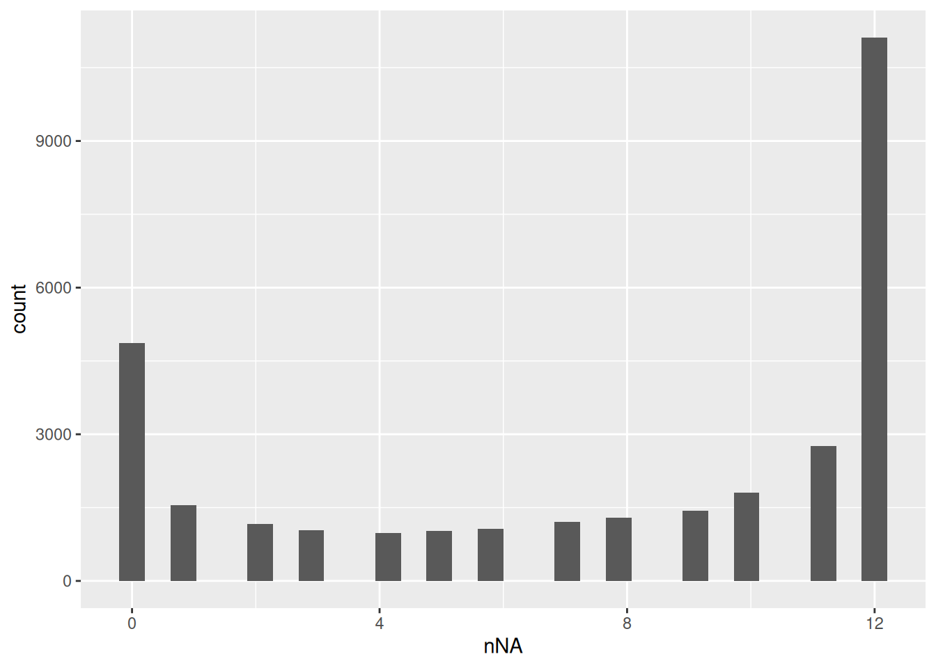

7.4.2 PSM filtering

We filter features based on 3 criteria (see PSM filtering).

1. Remove failed protein inference

We remove peptides that could not be uniquely mapped to a protein.

pe <- filterFeatures(pe,
  ~ Proteins != "" & ## Remove failed protein inference
    !grepl(";", Proteins)) ## Remove protein groups

'Proteins' found in 1 out of 1 assay(s).

2. Remove reverse sequences (decoys) and contaminants

We remove the contaminants and peptides that map to decoy sequences. These features bear no information of interest and will reduce the statistical power upon multiple test adjustment.

pe <- filterFeatures(pe, ~ Reverse != "+" & Potential.contaminant != "+")

'Reverse' found in 1 out of 1 assay(s).'Potential.contaminant' found in 1 out of 1 assay(s).

3. Remove highly missing peptides.

We keep peptides that were observed at last 3 times out of the \(n = 12\) samples, so we tolerate the following proportion of NAs: \(\text{pNA} = \frac{(n - 3)}{n} = 0.75\), so we keep peptides that are observed in at least 25% of the samples.

nObs <- 3
n <- ncol(pe[["peptides"]])
(pe <- filterNA(pe, i = "peptides", pNA = (n - nObs) / n))

An instance of class QFeatures (type: bulk) with 1 set:

 [1] peptides: SummarizedExperiment with 15630 rows and 12 columns 

We keep 15630 peptides upon filtering.

7.4.3 Identifications per sample

pe[,,"peptides"] |> 
  longForm(colvars = colnames(colData(pe)), 
           rowvars= c("Sequence", 
                      "Proteins")) |>
  data.frame() |>
  filter(!is.na(value)) |>
  group_by(location, tissue, sampleId) |>
  summarise(Precursors = length(unique(Sequence)),
            `Protein Groups` = length(unique(Proteins))) |> 
  pivot_longer(-(1:3),
               names_to = "Feature",
               values_to = "IDs") |> 
  ggplot(aes(x = sampleId, y = IDs, fill = interaction(location,tissue))) +
  geom_col() +
  #scale_fill_observable() +
  facet_wrap(~Feature,
             scales = "free_y") +
  labs(title = "Peptide and protein group identificiations per sample",
       x = "Sample",
       y = "Identifications") +
  theme_bw() + 
  theme(axis.text.x = element_text(angle = 90))

`summarise()` has regrouped the output.
ℹ Summaries were computed grouped by location, tissue, and sampleId.
ℹ Output is grouped by location and tissue.
ℹ Use `summarise(.groups = "drop_last")` to silence this message.
ℹ Use `summarise(.by = c(location, tissue, sampleId))` for per-operation
  grouping (`?dplyr::dplyr_by`) instead.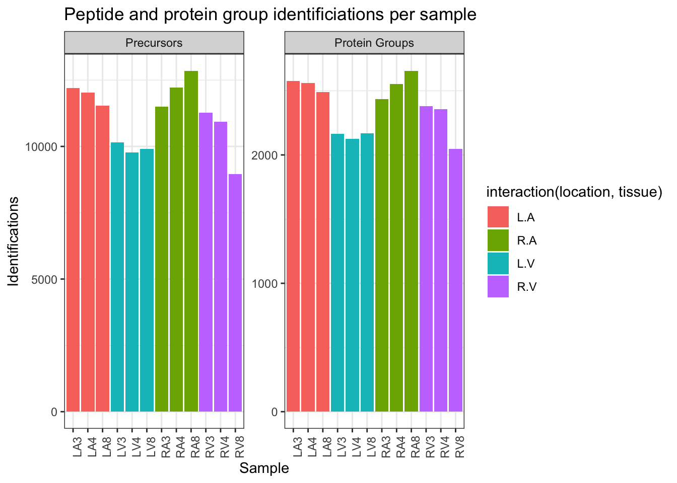

There are rather large variations in the peptide and protein identifications across samples. Therefore we will normalise the data using the Median of Ratios method of DESeq2, which can correct for differences in overall loading across runs as well as for differences in sample composition.

7.4.4 Standard preprocessing workflow

We can now prepare the data for modelling. The workflow ensures the data complies to msqrob2’s requirements:

1. Intensities are log-transformed.

pe <- logTransform(pe, base = 2, i = "peptides", name = "peptides_log")

2. Normalisation with Median of Ratios method.

pe <- sweep( #Subtract log2 norm factor column-by-column (MARGIN = 2)
  pe,
  MARGIN = 2,
  STATS = nfLogMedianOfRatios(pe,"peptides_log"),
  i = "peptides_log",
  name = "peptides_norm"
)

This function aims to calculate norm factors on a log scale, 
          the input data are assumed to be on the log-scale!

Upon the normalisation the density curves should be nicely centred. To confirm this, we will plot the intensity distributions for each biorepeat (mouse). longForm() seamlessly combines the quantification and annotation data into a table suitable for ggplot2 visualisation. We also subset the object with the data before and after normalisation.

longForm(pe[, , c("peptides_log", "peptides_norm")], colvar = "patient") |> 
  ggplot() +
  aes(x = value, group = colname, color = patient) +
  geom_density() +
  facet_wrap(~ assay, scale = "free")

Warning: 'experiments' dropped; see 'drops()'

harmonizing input:
  removing 12 sampleMap rows not in names(experiments)

Warning: Removed 108454 rows containing non-finite outside the scale range
(`stat_density()`).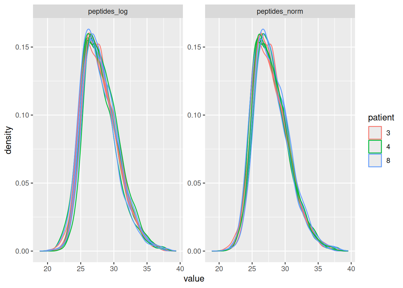

3. Summarisation to protein level.

We use the robust summary approach to infer protein-level data from peptide-level data, accounting for the fact that different peptides have ionisation efficiencies hence leading to different intensity baselines. As the robust summarisation takes a while we shift to medianPolish in this dataset.

pe <- aggregateFeatures(
  pe, i = "peptides_norm", fcol = "Proteins", 
  fun = MsCoreUtils::medianPolish, 
  na.rm = TRUE, name = "proteins"
)

Your quantitative and row data contain missing values. Please read the
relevant section(s) in the aggregateFeatures manual page regarding the
effects of missing values on data aggregation.

Aggregated: 1/1

7.5 Data exploration

We will explore the main sources of variation in the data using MDS.

library("scater")
se <- getWithColData(pe, "proteins") |> 
  as("SingleCellExperiment") |> 
  runMDS(exprs_values = 1) 

Warning: 'experiments' dropped; see 'drops()'

plotMDS(se, colour_by = "tissue") +
  plotMDS(se, colour_by = "location") +
  plotMDS(se, colour_by = "patient")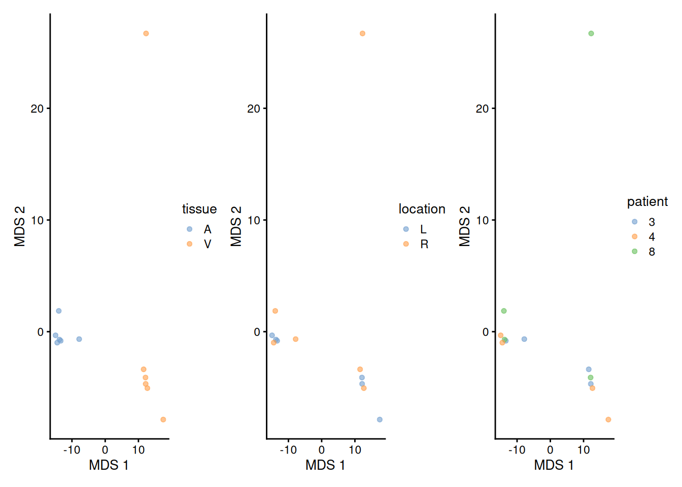

Note, that the samples upon robust summarisation show a clear separation according to the tissue type in the first dimension and according to location in the second dimension.

7.6 Data modelling

The preprocessed data can now be modelled to answer biologically relevant questions. Particularly, the protein abundance can differ according to tissue type (A-V) and location (L-R). Moreover, the effect of the tissue type can differ according to the location and vice versa. Hence, there can be an interaction between tissue and location.

The samples are also not independent as four biopsies (LA, RA, LV and RV) were taken for each patient. Because the proteome is profiled for each tissue x location combination within each patient, the design is a randomised complete block (RCB) design.

RCB designs can be correctly analysed by incorporating the block effect for patient either as a fixed or a random effect. The use of a fixed patient effect is here also possible because the effect of each factor combination can be estimated within block (patient).

Here, we choose to account for the patient effect using fixed effects because mixed models are computationally more demanding and rely on asymptotic inference (i.e. statistical inference is only valid for experiments with large sample sizes).

Now we have identified the sources of variation in the experiment that we have to account for (tissue, location and patient id), we can define a model.

model <- ~ location*tissue + ## (1) fixed effects: main effects for location and tissue type, and a tissue x location interaction
  patient  ## (2) fixed block effect for patient

7.6.1 Estimate the model

We estimate the model with msqrob(). Recall that variables defined in model are automatically retrieved from the colData (i.e. "tissue", "location", and "patient").

pe <- msqrob(
  pe, i = "proteins", formula = model, robust = TRUE
)

7.7 Statistical inference

Once the models are estimated, we can start answering biological questions by performing Statistical inference. We must translate the biological questions into a statistical hypotheses:

1. Is there an effect of tissue type (V-A) in the left heart region?
2. Is there an effect of tissue type (V-A) in the right heart region?
3. Is there on average an effect of tissue type in the heart.
4. Does the effect of tissue type (V-A) differ according to the heart region (L-R)?

In other words, we must translate these questions in a linear combination of the model parameters, also referred to as a contrast. To aid defining contrasts, we will visualise the experimental design using the ExploreModelMatrix package.

library("ExploreModelMatrix")
vd <- VisualizeDesign(
    sampleData =  colData(pe),
    designFormula = ~ location*tissue + patient,
    textSizeFitted = 4
)
vd$plotlist

$`location = L`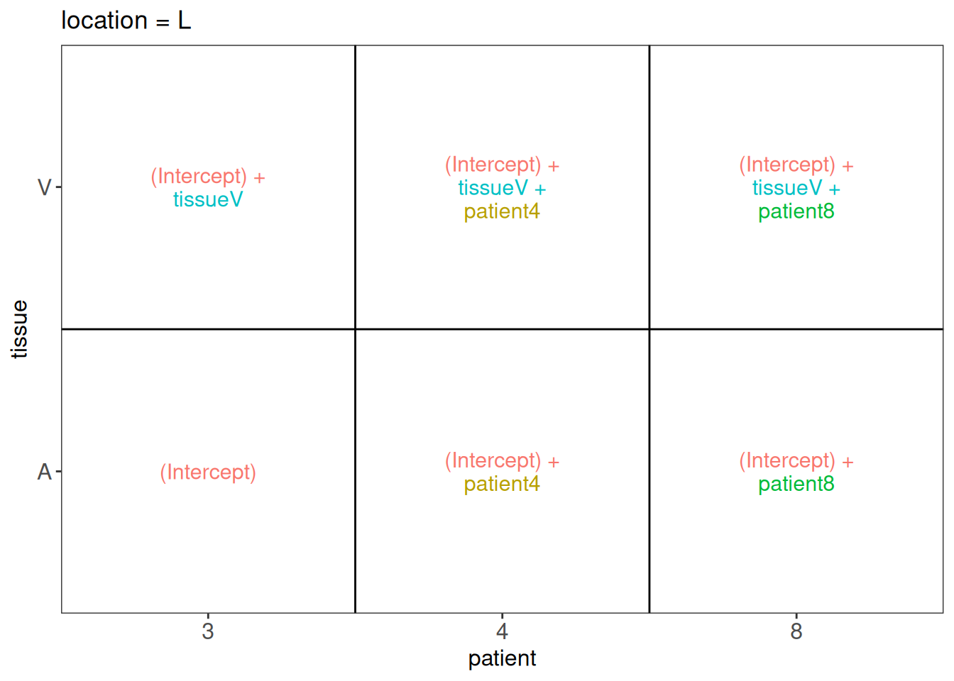

$`location = R`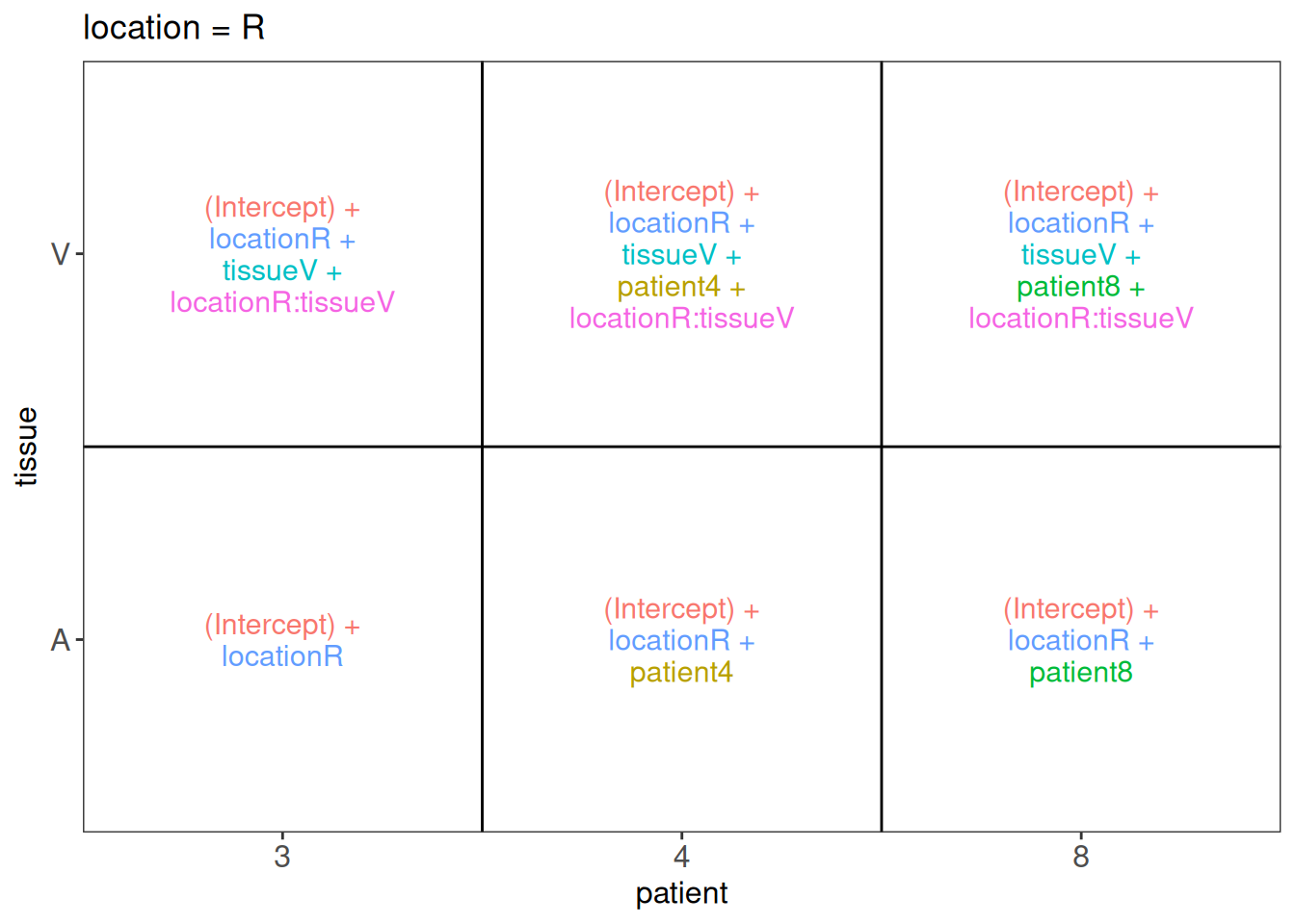

7.7.1 Research question 1: is there an effect of tissue in the left heart region?

From the plot we can see that the average log2 intensity for patient 3 in the left ventriculum equals `(Intercept) + tissueV’:

\[ \mu^L_{V,3} = \beta_0 + \beta_V \] and for the left atrium (Intercept):

\[ \mu^L_{A,3} = \beta_0 \] So the average \(\log_2 FC\) between atrium and ventriculum for patient 3 equals to parameter tissueV

\[ \log_2 FC_{V-A}^L = \mu^L_{V,3} -\mu^L_{A,3} = \beta_V \] The same can be seen for patient 4:

\[ \log_2 FC_{V-A}^L= \mu^L_{V,4} -\mu^L_{A,4} = \beta_0 + \beta_V + \beta_4 - (\beta_0 + \beta_4) = \beta_V \] So the parameter tissueV has the interpretation of the average \(\log_2 FC\) between ventriculum and atrium after correction for the patient effect, which quantifies the effect size for the first research hypothesis.

7.7.2 Research question 2: is there an effect of tissue in the right heart region?

When we use the same rationale for the right heart region, we can see that the average \(\log_2 FC\) between atrium and ventriculum upon correction for the patient effect equals tissueV + locationR:tissueV. So, it consists of the main effect for tissue and the location x tissue interaction.

We will illustrate this here for patient 4:

\[ \begin{array}{rcl} \log_2 FC_{V-A}^R& =&\mu^R_{V,4} -\mu^R_{A,4} \\ &=& \beta_0 + \beta_R + \beta_V + \beta_{R:V} + \beta_4 - (\beta_0 + \beta_R + \beta_4) \\ &=& \beta_V + \beta_{R:V} \end{array} \]

7.7.3 Research question 3: is there an effect of tissue on average in the heart?

This research question can be quantified by calculating the averaging the \(\log_2\) fold change between Ventriculum and Atrium over the left and right heart regions, which equals tissueV + 0.5*locationR:tissueV

\[ \begin{array}{rcl} (\log_2 FC_{V-A}^R + \log_2 FC_{V-A}^R)/ 2 &=& (\beta_V + \beta_V + \beta_{R:V})/2 \\ &=& \beta_V + 0.5\times\beta_{R:V} \end{array} \]

7.7.4 Research question 4: does the effect of tissue differs according to the heart region?

This research question can be quantified by calculating the difference in the \(\log_2\) fold change between Ventriculum and Atrium in the right and left heart regions, which equals locationR:tissueV

\[ \begin{array}{rcl} \log_2 FC_{V-A}^R- \log_2 FC_{V-A}^R &=& \beta_V + \beta_{R:V}-\beta_V \\ &=& \beta_{R:V} \end{array} \] ### Setting up the contrasts

We can set up the four contrasts:

1. We make the design matrix so that we can easily extract all parameter names from the model
2. We make the contrast matrix for the four contrasts

L <- makeContrast(
  c(
    "tissueV = 0",
    "tissueV + locationR:tissueV = 0",
    "tissueV + 0.5*locationR:tissueV = 0",
    "locationR:tissueV = 0"
  ),
  parameterNames = colnames(vd$designmatrix)
  )

We can now falsify the null hypothesis of each contrast:

pe <- hypothesisTest(
  object = pe, i = "proteins", contrast = L
)

7.7.5 Results tables for significant proteins

We first collect the results for all contrasts.

inferences <- 
  msqrobCollect(pe[["proteins"]], L) 
head(inferences)

                    logFC        se       df          t      pval   adjPval
tissueV.A0PJW6  0.8110076 0.5554057 8.288316  1.4602076 0.1810740 0.4251028
tissueV.A0PJZ3         NA        NA       NA         NA        NA        NA
tissueV.A0PK00         NA        NA       NA         NA        NA        NA
tissueV.A1A4S6  0.3414583 0.2889055 8.844266  1.1819029 0.2680461 0.5203615
tissueV.A1A5D9         NA        NA       NA         NA        NA        NA
tissueV.A1IGU5 -0.1769270 0.2931965 9.061510 -0.6034417 0.5610142 0.7774109
               contrast feature
tissueV.A0PJW6  tissueV  A0PJW6
tissueV.A0PJZ3  tissueV  A0PJZ3
tissueV.A0PK00  tissueV  A0PK00
tissueV.A1A4S6  tissueV  A1A4S6
tissueV.A1A5D9  tissueV  A1A5D9
tissueV.A1IGU5  tissueV  A1IGU5

Next, we will return tables of proteins for which the contrasts are significant at the 5% FDR level.

1. We set the significance level
2. We loop over the contrasts
3. We filter the significant results for the contrast from the table
4. We print the table

alpha <- 0.05 #1.
for (contrasti in colnames(L)) #2. 
{
  sigList <- inferences |> 
    filter(contrast == contrasti & adjPval < alpha) #3.
  cat("**Contrast:**", contrasti, "= 0 (", nrow(sigList), " significant proteins)\n\n") #4.
  print(kable(sigList, row.names = FALSE) |>
      kable_styling(full_width = FALSE) |>
      scroll_box(height = "250px")
      ) #4.
  cat("\n\n\n---\n\n") #4.
}

Contrast: tissueV = 0 ( 84 significant proteins)

logFC	se	df	t	pval	adjPval	contrast	feature
-3.916945	0.7741480	8.157297	-5.059685	0.0009211	0.0338517	tissueV	O00180
-2.044625	0.3171714	8.859530	-6.446435	0.0001272	0.0174679	tissueV	O14967
-2.379147	0.4431350	8.881741	-5.368899	0.0004717	0.0270688	tissueV	O43677
-3.280059	0.6182246	8.157297	-5.305611	0.0006786	0.0304450	tissueV	O60760
-1.844500	0.2836538	9.128979	-6.502646	0.0001042	0.0174679	tissueV	O75368
2.258082	0.4916897	8.829633	4.592494	0.0013710	0.0428517	tissueV	O75394
1.827648	0.4004574	8.834504	4.563902	0.0014252	0.0428517	tissueV	O75629
2.743133	0.3435029	8.175631	7.985763	0.0000391	0.0112822	tissueV	O94875-10
-3.763413	0.5377865	5.157297	-6.997967	0.0008082	0.0319941	tissueV	O95631
-1.693278	0.3078980	8.911848	-5.499475	0.0003939	0.0265062	tissueV	O95865
-2.004354	0.4258027	8.674862	-4.707238	0.0012256	0.0399100	tissueV	O95980
-1.756089	0.3012493	8.357695	-5.829355	0.0003320	0.0265062	tissueV	P00325
-3.927443	0.6584614	6.087571	-5.964575	0.0009438	0.0338517	tissueV	P01699
-2.337834	0.4070974	8.893943	-5.742688	0.0002916	0.0260534	tissueV	P02452
-1.774119	0.3349219	9.157297	-5.297111	0.0004680	0.0270688	tissueV	P02743
-2.585440	0.3822816	7.952607	-6.763182	0.0001471	0.0174679	tissueV	P02747
-1.663394	0.3702070	9.157297	-4.493146	0.0014398	0.0428517	tissueV	P02775
-1.240956	0.2679630	9.079099	-4.631073	0.0012065	0.0399100	tissueV	P04083
-1.527743	0.2987129	9.016618	-5.114419	0.0006291	0.0303099	tissueV	P04196
1.699180	0.3427136	8.989012	4.958019	0.0007855	0.0319941	tissueV	P04209
-1.613522	0.2552800	9.088096	-6.320597	0.0001319	0.0174679	tissueV	P05546
-2.676909	0.4821749	8.820475	-5.551740	0.0003821	0.0265062	tissueV	P05997
2.084096	0.3607958	9.109713	5.776387	0.0002552	0.0257672	tissueV	P06858
-2.327282	0.3629198	8.827747	-6.412661	0.0001344	0.0174679	tissueV	P08294
-1.503653	0.3110420	9.007195	-4.834246	0.0009263	0.0338517	tissueV	P08582
8.356406	0.4753349	9.157297	17.580038	0.0000000	0.0000461	tissueV	P08590
7.258000	0.4982727	7.157297	14.566321	0.0000014	0.0009417	tissueV	P10916
4.827314	0.3759382	9.016980	12.840711	0.0000004	0.0004280	tissueV	P12883
-3.717134	0.6489652	8.895961	-5.727786	0.0002968	0.0260534	tissueV	P13533
2.399958	0.2553933	8.847548	9.397109	0.0000068	0.0034090	tissueV	P14854
1.082278	0.2440195	8.974688	4.435210	0.0016461	0.0442072	tissueV	P14923
1.538482	0.2769236	8.486002	5.555620	0.0004363	0.0268344	tissueV	P15924
1.288628	0.2894122	8.876133	4.452567	0.0016497	0.0442072	tissueV	P17540
-1.863036	0.3031679	8.835976	-6.145231	0.0001832	0.0205453	tissueV	P18428
2.871955	0.5226915	8.819226	5.494551	0.0004112	0.0267778	tissueV	P19429
-2.710880	0.4033576	8.683908	-6.720785	0.0001023	0.0174679	tissueV	P21810
-3.889514	0.6158707	7.157297	-6.315472	0.0003636	0.0265062	tissueV	P23083
1.494665	0.2926712	9.157297	5.106976	0.0006054	0.0303099	tissueV	P23434
1.663250	0.3761258	8.684232	4.422057	0.0018177	0.0453389	tissueV	P24298
2.128221	0.3693180	9.154332	5.762572	0.0002550	0.0257672	tissueV	P24311
-2.192662	0.3752983	8.671591	-5.842451	0.0002839	0.0260534	tissueV	P24844
-1.592623	0.2717608	8.348854	-5.860384	0.0003214	0.0265062	tissueV	P29622
1.686612	0.3758292	9.020472	4.487710	0.0015069	0.0428517	tissueV	P35754
-2.753027	0.5251033	8.157297	-5.242829	0.0007331	0.0309572	tissueV	P36021
-1.981308	0.3793378	8.965158	-5.223071	0.0005539	0.0292481	tissueV	P36955
-1.787446	0.2667411	9.066468	-6.701052	0.0000854	0.0174679	tissueV	P46821
-1.832345	0.3635804	9.027078	-5.039726	0.0006936	0.0304450	tissueV	P51884
-2.724376	0.3524021	8.660008	-7.730874	0.0000361	0.0112822	tissueV	P51888
1.552464	0.3269019	9.157297	4.749022	0.0009967	0.0338517	tissueV	Q00G26
-4.100799	0.7909636	8.723814	-5.184561	0.0006362	0.0303099	tissueV	Q06828
1.488165	0.3133790	9.127855	4.748771	0.0010060	0.0338517	tissueV	Q13011
-1.193748	0.2511842	9.157297	-4.752482	0.0009918	0.0338517	tissueV	Q14764
-2.161374	0.3921764	9.157297	-5.511229	0.0003524	0.0265062	tissueV	Q15113
-2.216355	0.4146662	8.901511	-5.344913	0.0004830	0.0270688	tissueV	Q16647
-2.075418	0.3882397	9.157297	-5.345713	0.0004386	0.0268344	tissueV	Q53GQ0
-3.200391	0.6828882	8.157297	-4.686551	0.0014884	0.0428517	tissueV	Q5M9N0
-1.939256	0.4268946	8.412932	-4.542704	0.0016641	0.0442072	tissueV	Q5NDL2
-2.264859	0.4704839	7.157297	-4.813892	0.0018189	0.0453389	tissueV	Q6SZW1
-2.945962	0.3443276	8.776411	-8.555695	0.0000151	0.0061063	tissueV	Q6UWY5
1.475862	0.3169896	8.003863	4.655868	0.0016301	0.0442072	tissueV	Q6YN16
1.797598	0.3974191	8.939663	4.523180	0.0014650	0.0428517	tissueV	Q86VU5
-2.936360	0.3957069	7.865352	-7.420541	0.0000816	0.0174679	tissueV	Q8N474
-2.356973	0.3798247	9.157297	-6.205423	0.0001467	0.0174679	tissueV	Q8TBQ9
-5.327875	1.0032217	8.266154	-5.310765	0.0006455	0.0303099	tissueV	Q8WWA0
1.115818	0.2563529	9.110666	4.352664	0.0017906	0.0453389	tissueV	Q8WZ42-6
-2.963445	0.6424629	8.671141	-4.612632	0.0013977	0.0428517	tissueV	Q92736-2
1.902891	0.4193664	8.165125	4.537538	0.0018086	0.0453389	tissueV	Q96FJ2
-2.720096	0.5222524	6.129965	-5.208393	0.0018721	0.0456538	tissueV	Q96H79
-2.008136	0.4128901	8.713368	-4.863610	0.0009784	0.0338517	tissueV	Q96LL9
-2.401282	0.4477225	8.768946	-5.363327	0.0004961	0.0270688	tissueV	Q9BW30
-2.290433	0.5208671	8.871291	-4.397346	0.0017880	0.0453389	tissueV	Q9BXN1
1.948862	0.4190949	8.645959	4.650169	0.0013374	0.0428517	tissueV	Q9BXV9
2.529876	0.5698865	8.157297	4.439264	0.0020688	0.0497242	tissueV	Q9NRG4
-5.672898	0.8264728	5.157297	-6.863987	0.0008855	0.0338517	tissueV	Q9NVN8
-1.941685	0.4074266	9.157297	-4.765731	0.0009734	0.0338517	tissueV	Q9NZ01
-1.795959	0.3278928	9.157297	-5.477276	0.0003685	0.0265062	tissueV	Q9P2B2
-2.069165	0.4142186	9.031128	-4.995346	0.0007360	0.0309572	tissueV	Q9UBG0
-1.876394	0.4152614	9.003376	-4.518585	0.0014484	0.0428517	tissueV	Q9UGT4
1.752743	0.3376941	8.505605	5.190328	0.0006847	0.0304450	tissueV	Q9UKS6
-2.223787	0.4205438	7.787547	-5.287884	0.0008069	0.0319941	tissueV	Q9UL18
-3.081151	0.4292045	7.996682	-7.178748	0.0000946	0.0174679	tissueV	Q9ULL5-3
3.972042	0.7597053	8.891134	5.228397	0.0005650	0.0292481	tissueV	Q9UNW9
1.125299	0.2609266	9.157297	4.312702	0.0018768	0.0456538	tissueV	Q9Y4W6
-3.786973	0.8534131	8.988851	-4.437445	0.0016345	0.0442072	tissueV	Q9Y5U8

---

Contrast: tissueV + locationR:tissueV = 0 ( 52 significant proteins)

logFC	se	df	t	pval	adjPval	contrast	feature
1.678458	0.3055067	8.448267	5.494012	0.0004781	0.0381366	tissueV + locationR:tissueV	A6NDG6
-2.762249	0.5229097	8.950421	-5.282459	0.0005148	0.0394557	tissueV + locationR:tissueV	A6NMZ7
-4.414052	0.8939092	8.157297	-4.937919	0.0010748	0.0478520	tissueV + locationR:tissueV	O00180
-2.664358	0.4524752	8.881741	-5.888407	0.0002447	0.0325294	tissueV + locationR:tissueV	O43677
-1.401117	0.2831188	9.128979	-4.948866	0.0007598	0.0454250	tissueV + locationR:tissueV	O75368
-1.288679	0.2728096	8.867625	-4.723729	0.0011283	0.0478520	tissueV + locationR:tissueV	P01031
-1.788018	0.3702070	9.157297	-4.829778	0.0008892	0.0454250	tissueV + locationR:tissueV	P02775
-2.489397	0.3283460	8.756467	-7.581626	0.0000394	0.0196514	tissueV + locationR:tissueV	P02776
-1.693975	0.3099743	8.929917	-5.464889	0.0004089	0.0339709	tissueV + locationR:tissueV	P04004
-1.412195	0.2537686	9.088096	-5.564893	0.0003377	0.0339709	tissueV + locationR:tissueV	P05546
3.783171	0.3593391	9.109713	10.528135	0.0000021	0.0021077	tissueV + locationR:tissueV	P06858
-1.726551	0.3537382	8.827747	-4.880871	0.0009204	0.0454250	tissueV + locationR:tissueV	P08294
5.569744	0.4753349	9.157297	11.717514	0.0000008	0.0016142	tissueV + locationR:tissueV	P08590
3.170748	0.4982727	7.157297	6.363479	0.0003470	0.0339709	tissueV + locationR:tissueV	P10916
2.378103	0.3620366	7.831728	6.568682	0.0001923	0.0316263	tissueV + locationR:tissueV	P11586
2.030950	0.3712980	9.016980	5.469867	0.0003927	0.0339709	tissueV + locationR:tissueV	P12883
-3.482735	0.6332942	8.895961	-5.499395	0.0003964	0.0339709	tissueV + locationR:tissueV	P13533
1.276035	0.2630781	8.847548	4.850405	0.0009534	0.0454250	tissueV + locationR:tissueV	P14854
-2.489020	0.3881798	8.683908	-6.412028	0.0001446	0.0265417	tissueV + locationR:tissueV	P21810
-2.496573	0.5197684	8.227272	-4.803242	0.0012479	0.0478520	tissueV + locationR:tissueV	P23142
1.735443	0.2926712	9.157297	5.929667	0.0002062	0.0316263	tissueV + locationR:tissueV	P23434
1.255834	0.2415012	9.152482	5.200117	0.0005343	0.0394557	tissueV + locationR:tissueV	P23786
2.526379	0.3946987	8.684232	6.400779	0.0001464	0.0265417	tissueV + locationR:tissueV	P24298
-1.851478	0.3286891	9.016492	-5.632914	0.0003184	0.0339709	tissueV + locationR:tissueV	P28066
-1.856030	0.3707771	7.728301	-5.005784	0.0011591	0.0478520	tissueV + locationR:tissueV	P30711
-3.580403	0.6784715	6.923640	-5.277160	0.0011926	0.0478520	tissueV + locationR:tissueV	P35625
-2.816136	0.3487907	8.851985	-8.074001	0.0000227	0.0150814	tissueV + locationR:tissueV	P48163
-1.583932	0.3362634	8.660008	-4.710390	0.0012260	0.0478520	tissueV + locationR:tissueV	P51888
-2.444671	0.3528478	9.157297	-6.928403	0.0000629	0.0208937	tissueV + locationR:tissueV	P54652
-2.095858	0.3453810	7.901822	-6.068250	0.0003149	0.0339709	tissueV + locationR:tissueV	P60468
2.252143	0.4303035	7.638694	5.233848	0.0009151	0.0454250	tissueV + locationR:tissueV	P61925
2.325532	0.3269019	9.157297	7.113852	0.0000511	0.0203783	tissueV + locationR:tissueV	Q00G26
2.535090	0.4134774	8.442103	6.131145	0.0002247	0.0320040	tissueV + locationR:tissueV	Q04760
-3.841336	0.7578337	8.723814	-5.068838	0.0007408	0.0454250	tissueV + locationR:tissueV	Q06828
-1.793274	0.3289927	9.153218	-5.450801	0.0003822	0.0339709	tissueV + locationR:tissueV	Q15327
2.003012	0.4206893	9.157297	4.761261	0.0009796	0.0454250	tissueV + locationR:tissueV	Q53GG5
-2.439944	0.4622848	8.412932	-5.278010	0.0006346	0.0421829	tissueV + locationR:tissueV	Q5NDL2
3.630809	0.5725894	8.822615	6.341034	0.0001464	0.0265417	tissueV + locationR:tissueV	Q69YU5
-1.934958	0.3879279	8.241167	-4.987931	0.0009782	0.0454250	tissueV + locationR:tissueV	Q6PCB0
2.146536	0.4385193	8.736894	4.894962	0.0009305	0.0454250	tissueV + locationR:tissueV	Q6PI78
-2.215743	0.3315729	8.776411	-6.682521	0.0001016	0.0265417	tissueV + locationR:tissueV	Q6UWY5
1.879984	0.3419166	8.003863	5.498372	0.0005739	0.0408690	tissueV + locationR:tissueV	Q6YN16
1.616618	0.3413864	8.578279	4.735451	0.0012160	0.0478520	tissueV + locationR:tissueV	Q8N142
-2.410524	0.4806043	7.840129	-5.015611	0.0010970	0.0478520	tissueV + locationR:tissueV	Q92930
3.058707	0.5938612	8.157297	5.150542	0.0008220	0.0454250	tissueV + locationR:tissueV	Q96MM6
3.194926	0.5720793	6.893659	5.584760	0.0008741	0.0454250	tissueV + locationR:tissueV	Q9BSD7
2.214363	0.4426004	8.924131	5.003075	0.0007549	0.0454250	tissueV + locationR:tissueV	Q9HAT2
2.846025	0.4935361	8.157297	5.766599	0.0003915	0.0339709	tissueV + locationR:tissueV	Q9NRG4
1.813177	0.3909000	9.015740	4.638469	0.0012163	0.0478520	tissueV + locationR:tissueV	Q9NRX4
-1.595232	0.3278928	9.157297	-4.865101	0.0008462	0.0454250	tissueV + locationR:tissueV	Q9P2B2
-2.159706	0.4209924	9.003376	-5.130036	0.0006188	0.0421829	tissueV + locationR:tissueV	Q9UGT4
-3.155415	0.3742516	6.065295	-8.431266	0.0001434	0.0265417	tissueV + locationR:tissueV	Q9ULD0

---

Contrast: tissueV + 0.5 * locationR:tissueV = 0 ( 275 significant proteins)

logFC	se	df	t	pval	adjPval	contrast	feature
-1.8305581	0.4492633	7.378127	-4.074577	0.0042244	0.0384467	tissueV + 0.5 * locationR:tissueV	A5D6W6
1.5090670	0.2178204	8.448267	6.928032	0.0000932	0.0050239	tissueV + 0.5 * locationR:tissueV	A6NDG6
-2.3762212	0.3732261	8.950421	-6.366707	0.0001335	0.0059539	tissueV + 0.5 * locationR:tissueV	A6NMZ7
1.5175637	0.3500645	7.558249	4.335097	0.0028520	0.0304112	tissueV + 0.5 * locationR:tissueV	I3L505
0.7853044	0.2165607	9.157297	3.626256	0.0053616	0.0424249	tissueV + 0.5 * locationR:tissueV	O00151
-4.1654985	0.5912653	8.157297	-7.045058	0.0000980	0.0051365	tissueV + 0.5 * locationR:tissueV	O00180
-1.0261781	0.2593393	8.516375	-3.956893	0.0037037	0.0362022	tissueV + 0.5 * locationR:tissueV	O00264
1.8997136	0.4503359	7.008993	4.218437	0.0039329	0.0377028	tissueV + 0.5 * locationR:tissueV	O14531
1.3446890	0.3826579	8.852081	3.514076	0.0067483	0.0494707	tissueV + 0.5 * locationR:tissueV	O14558
1.2215442	0.2687123	9.117663	4.545919	0.0013485	0.0218607	tissueV + 0.5 * locationR:tissueV	O14949
-1.3275191	0.2257962	8.859530	-5.879281	0.0002499	0.0081709	tissueV + 0.5 * locationR:tissueV	O14967
-0.6500399	0.1676996	9.157297	-3.876216	0.0036318	0.0356740	tissueV + 0.5 * locationR:tissueV	O14980
-1.8040348	0.4115718	6.157297	-4.383281	0.0043748	0.0391004	tissueV + 0.5 * locationR:tissueV	O15118
-0.9243018	0.1941962	8.432683	-4.759630	0.0012340	0.0206769	tissueV + 0.5 * locationR:tissueV	O15230
-1.7434130	0.4553898	8.823556	-3.828397	0.0041885	0.0384467	tissueV + 0.5 * locationR:tissueV	O43175
-2.5217527	0.3166727	8.881741	-7.963278	0.0000248	0.0029497	tissueV + 0.5 * locationR:tissueV	O43677
0.9596508	0.2675196	8.847038	3.587217	0.0060299	0.0457169	tissueV + 0.5 * locationR:tissueV	O43678
1.0309632	0.2344069	9.106355	4.398178	0.0016768	0.0235457	tissueV + 0.5 * locationR:tissueV	O43920
1.7231972	0.3244189	6.157297	5.311642	0.0016686	0.0235457	tissueV + 0.5 * locationR:tissueV	O60503
-1.9045043	0.4089171	8.157297	-4.657433	0.0015465	0.0231859	tissueV + 0.5 * locationR:tissueV	O60760
1.5653993	0.3636393	9.157297	4.304813	0.0018989	0.0242697	tissueV + 0.5 * locationR:tissueV	O75190-3
-1.6228085	0.2003842	9.128979	-8.098484	0.0000184	0.0029497	tissueV + 0.5 * locationR:tissueV	O75368
1.3495773	0.3533083	8.829633	3.819829	0.0042378	0.0384467	tissueV + 0.5 * locationR:tissueV	O75394
1.1492265	0.2158775	8.975527	5.323511	0.0004831	0.0121947	tissueV + 0.5 * locationR:tissueV	O75489
-1.0383752	0.2690520	9.157297	-3.859384	0.0037274	0.0362556	tissueV + 0.5 * locationR:tissueV	O75828
0.7705458	0.2110944	9.154332	3.650243	0.0051659	0.0423992	tissueV + 0.5 * locationR:tissueV	O75947
0.6667616	0.1792853	9.157297	3.718998	0.0046358	0.0407217	tissueV + 0.5 * locationR:tissueV	O76031
2.1115014	0.2546417	8.175631	8.292047	0.0000296	0.0032112	tissueV + 0.5 * locationR:tissueV	O94875-10
-0.7426045	0.1785123	9.111675	-4.159963	0.0023831	0.0274679	tissueV + 0.5 * locationR:tissueV	O94919
0.9552882	0.2158298	9.064751	4.426119	0.0016277	0.0234736	tissueV + 0.5 * locationR:tissueV	O95182
0.6495623	0.1796247	9.044044	3.616219	0.0055598	0.0432021	tissueV + 0.5 * locationR:tissueV	O95202
-2.1673562	0.5700161	9.116164	-3.802272	0.0041055	0.0384467	tissueV + 0.5 * locationR:tissueV	O95445
-1.2481692	0.2189883	8.911848	-5.699706	0.0003054	0.0092266	tissueV + 0.5 * locationR:tissueV	O95865
-1.5817805	0.2969965	8.674862	-5.325924	0.0005396	0.0130605	tissueV + 0.5 * locationR:tissueV	O95980
-1.1718628	0.2229353	8.357695	-5.256515	0.0006662	0.0145976	tissueV + 0.5 * locationR:tissueV	P00325
-0.7676860	0.1997066	8.744291	-3.844070	0.0041601	0.0384467	tissueV + 0.5 * locationR:tissueV	P00352
-1.4371418	0.2857187	8.816868	-5.029919	0.0007553	0.0153677	tissueV + 0.5 * locationR:tissueV	P00748
-1.1792764	0.3178507	9.157297	-3.710158	0.0047003	0.0409760	tissueV + 0.5 * locationR:tissueV	P01008
-0.7051905	0.1889061	8.688920	-3.733021	0.0049750	0.0418571	tissueV + 0.5 * locationR:tissueV	P01024
-1.1289301	0.1921210	8.867625	-5.876142	0.0002500	0.0081709	tissueV + 0.5 * locationR:tissueV	P01031
-1.1935163	0.2668628	8.690200	-4.472397	0.0016903	0.0235694	tissueV + 0.5 * locationR:tissueV	P01034
-2.1723594	0.4373143	7.157297	-4.967501	0.0015217	0.0229867	tissueV + 0.5 * locationR:tissueV	P01042
-1.8448050	0.2868406	8.893943	-6.431463	0.0001272	0.0059007	tissueV + 0.5 * locationR:tissueV	P02452
-2.5362556	0.5822867	8.116412	-4.355682	0.0023448	0.0271975	tissueV + 0.5 * locationR:tissueV	P02461
-1.5151210	0.2368256	9.157297	-6.397624	0.0001164	0.0055520	tissueV + 0.5 * locationR:tissueV	P02743
-1.6498886	0.2548336	7.952607	-6.474376	0.0001983	0.0074615	tissueV + 0.5 * locationR:tissueV	P02747
-0.9752747	0.2149219	8.499267	-4.537809	0.0016321	0.0234736	tissueV + 0.5 * locationR:tissueV	P02748
-1.7257058	0.2617759	9.157297	-6.592303	0.0000925	0.0050239	tissueV + 0.5 * locationR:tissueV	P02775
-1.9398419	0.2364330	8.756467	-8.204614	0.0000213	0.0029497	tissueV + 0.5 * locationR:tissueV	P02776
-1.0189097	0.2451977	8.906264	-4.155461	0.0025209	0.0283996	tissueV + 0.5 * locationR:tissueV	P02790
0.9530644	0.2314715	8.941487	4.117415	0.0026445	0.0291335	tissueV + 0.5 * locationR:tissueV	P03928
-1.3389431	0.3373665	9.047906	-3.968809	0.0032263	0.0329911	tissueV + 0.5 * locationR:tissueV	P03950
-1.1775644	0.2431514	9.102361	-4.842926	0.0008881	0.0170277	tissueV + 0.5 * locationR:tissueV	P04003
-1.4339388	0.2169264	8.929917	-6.610256	0.0001017	0.0051365	tissueV + 0.5 * locationR:tissueV	P04004
-1.0216923	0.1888435	9.079099	-5.410260	0.0004146	0.0108777	tissueV + 0.5 * locationR:tissueV	P04083
-1.3295815	0.2099189	9.016618	-6.333787	0.0001344	0.0059539	tissueV + 0.5 * locationR:tissueV	P04196
0.9696338	0.2441200	8.989012	3.971956	0.0032529	0.0330935	tissueV + 0.5 * locationR:tissueV	P04209
-0.8259305	0.2201554	8.297707	-3.751580	0.0052540	0.0423992	tissueV + 0.5 * locationR:tissueV	P04275
-1.5128585	0.1799766	9.088096	-8.405860	0.0000140	0.0027908	tissueV + 0.5 * locationR:tissueV	P05546
-2.1936811	0.3355684	8.820475	-6.537210	0.0001169	0.0055520	tissueV + 0.5 * locationR:tissueV	P05997
-0.7889658	0.2144433	8.106256	-3.679134	0.0060858	0.0458141	tissueV + 0.5 * locationR:tissueV	P06727
0.8761177	0.2048871	8.100287	4.276099	0.0026255	0.0290842	tissueV + 0.5 * locationR:tissueV	P06732
2.9336337	0.2546067	9.109713	11.522218	0.0000010	0.0005369	tissueV + 0.5 * locationR:tissueV	P06858
1.1061473	0.2134874	9.107539	5.181324	0.0005567	0.0130605	tissueV + 0.5 * locationR:tissueV	P07195
-0.7432135	0.2046665	9.157297	-3.631339	0.0053189	0.0423992	tissueV + 0.5 * locationR:tissueV	P07357
-0.8542467	0.2166916	8.713301	-3.942223	0.0036174	0.0356740	tissueV + 0.5 * locationR:tissueV	P07451
-1.7846803	0.3724007	8.830490	-4.792365	0.0010381	0.0191662	tissueV + 0.5 * locationR:tissueV	P07585
0.9511707	0.2583519	7.716859	3.681686	0.0066068	0.0487924	tissueV + 0.5 * locationR:tissueV	P07686
-2.0269162	0.2534125	8.827747	-7.998487	0.0000248	0.0029497	tissueV + 0.5 * locationR:tissueV	P08294
0.7158309	0.1896845	9.157297	3.773798	0.0042562	0.0384467	tissueV + 0.5 * locationR:tissueV	P08574
6.9630751	0.3361126	9.157297	20.716498	0.0000000	0.0000105	tissueV + 0.5 * locationR:tissueV	P08590
-0.8458615	0.2216663	9.157297	-3.815923	0.0039867	0.0378544	tissueV + 0.5 * locationR:tissueV	P08603
-0.7211043	0.1934998	8.397901	-3.726642	0.0053350	0.0423992	tissueV + 0.5 * locationR:tissueV	P09619
0.6571505	0.1791290	9.153550	3.668589	0.0050200	0.0418826	tissueV + 0.5 * locationR:tissueV	P09874
1.2652262	0.2142713	9.132053	5.904787	0.0002150	0.0076418	tissueV + 0.5 * locationR:tissueV	P10109
5.2143738	0.3447541	7.157297	15.124909	0.0000011	0.0005369	tissueV + 0.5 * locationR:tissueV	P10916
0.7422891	0.2023671	8.924330	3.668032	0.0052453	0.0423992	tissueV + 0.5 * locationR:tissueV	P11182
1.6230884	0.2414080	7.831728	6.723425	0.0001643	0.0065383	tissueV + 0.5 * locationR:tissueV	P11586
0.9043326	0.1954401	9.050014	4.627159	0.0012236	0.0206769	tissueV + 0.5 * locationR:tissueV	P11766
-1.1168778	0.2430773	7.817062	-4.594743	0.0018773	0.0242697	tissueV + 0.5 * locationR:tissueV	P12110
-1.6249193	0.3040220	7.965384	-5.344742	0.0007002	0.0151759	tissueV + 0.5 * locationR:tissueV	P12814
3.4291320	0.2641930	9.016980	12.979648	0.0000004	0.0003853	tissueV + 0.5 * locationR:tissueV	P12883
0.8611279	0.1982061	9.054875	4.344608	0.0018383	0.0242697	tissueV + 0.5 * locationR:tissueV	P13073
-3.5999343	0.4533810	8.895961	-7.940197	0.0000251	0.0029497	tissueV + 0.5 * locationR:tissueV	P13533
-0.8161822	0.1895501	9.080490	-4.305891	0.0019332	0.0243977	tissueV + 0.5 * locationR:tissueV	P13667
-1.0213627	0.2422175	9.157297	-4.216718	0.0021651	0.0261648	tissueV + 0.5 * locationR:tissueV	P13671
-1.0202344	0.2257367	8.937862	-4.519577	0.0014733	0.0229867	tissueV + 0.5 * locationR:tissueV	P14543
-0.8817506	0.1937042	8.815088	-4.552047	0.0014575	0.0229867	tissueV + 0.5 * locationR:tissueV	P14550
1.8379968	0.1833274	8.847548	10.025759	0.0000040	0.0013235	tissueV + 0.5 * locationR:tissueV	P14854
0.8708156	0.1739866	8.974688	5.005073	0.0007401	0.0153677	tissueV + 0.5 * locationR:tissueV	P14923
1.0974948	0.2922507	7.179366	3.755320	0.0067963	0.0496406	tissueV + 0.5 * locationR:tissueV	P15374
1.2031555	0.2867251	8.153493	4.196199	0.0028875	0.0306241	tissueV + 0.5 * locationR:tissueV	P15848
1.2317458	0.1896515	8.486002	6.494785	0.0001458	0.0061875	tissueV + 0.5 * locationR:tissueV	P15924
0.9441956	0.2449053	8.697577	3.855350	0.0041318	0.0384467	tissueV + 0.5 * locationR:tissueV	P16219
-0.7496100	0.1979110	9.091662	-3.787611	0.0042203	0.0384467	tissueV + 0.5 * locationR:tissueV	P17050
1.1665903	0.2351265	7.673684	4.961543	0.0012491	0.0207560	tissueV + 0.5 * locationR:tissueV	P17174
1.1794532	0.2074162	8.876133	5.686408	0.0003152	0.0092656	tissueV + 0.5 * locationR:tissueV	P17540
-1.5335655	0.2164079	8.835976	-7.086457	0.0000631	0.0044944	tissueV + 0.5 * locationR:tissueV	P18428
2.5940289	0.3636839	8.819226	7.132647	0.0000606	0.0044781	tissueV + 0.5 * locationR:tissueV	P19429
-1.6390054	0.3678883	8.664047	-4.455171	0.0017447	0.0238285	tissueV + 0.5 * locationR:tissueV	P20774
0.8187813	0.1750712	9.157297	4.676847	0.0011046	0.0198433	tissueV + 0.5 * locationR:tissueV	P21399
-2.5999497	0.2798430	8.683908	-9.290743	0.0000084	0.0023998	tissueV + 0.5 * locationR:tissueV	P21810
0.8381284	0.2131661	9.037377	3.931809	0.0034208	0.0342841	tissueV + 0.5 * locationR:tissueV	P22695
1.6782826	0.4120514	8.487366	4.072993	0.0031513	0.0323898	tissueV + 0.5 * locationR:tissueV	P22748
-2.8984783	0.4548507	7.157297	-6.372373	0.0003440	0.0098676	tissueV + 0.5 * locationR:tissueV	P23083
-2.1422747	0.3526376	8.227272	-6.075004	0.0002660	0.0084178	tissueV + 0.5 * locationR:tissueV	P23142
1.6150539	0.2069498	9.157297	7.804085	0.0000244	0.0029497	tissueV + 0.5 * locationR:tissueV	P23434
0.9316577	0.1707328	9.152482	5.456817	0.0003792	0.0103591	tissueV + 0.5 * locationR:tissueV	P23786
2.0948144	0.2726067	8.684232	7.684384	0.0000372	0.0035325	tissueV + 0.5 * locationR:tissueV	P24298
1.4373722	0.2611150	9.154332	5.504748	0.0003558	0.0099939	tissueV + 0.5 * locationR:tissueV	P24311
1.0430828	0.2335958	9.126340	4.465332	0.0015120	0.0229867	tissueV + 0.5 * locationR:tissueV	P24752
-1.8174310	0.2599221	8.671591	-6.992215	0.0000767	0.0049327	tissueV + 0.5 * locationR:tissueV	P24844
-1.2172955	0.2659794	8.324610	-4.576654	0.0016329	0.0234736	tissueV + 0.5 * locationR:tissueV	P25940
1.8921754	0.4597960	9.005651	4.115250	0.0026129	0.0290842	tissueV + 0.5 * locationR:tissueV	P27144
-1.2806296	0.2338805	9.016492	-5.475572	0.0003899	0.0103663	tissueV + 0.5 * locationR:tissueV	P28066
-1.4641296	0.1959590	8.348854	-7.471612	0.0000569	0.0043616	tissueV + 0.5 * locationR:tissueV	P29622
-1.3149681	0.2704919	9.088423	-4.861395	0.0008693	0.0169939	tissueV + 0.5 * locationR:tissueV	P30405
-1.5213926	0.2820692	7.728301	-5.393685	0.0007309	0.0153677	tissueV + 0.5 * locationR:tissueV	P30711
0.7346926	0.1935212	8.476450	3.796445	0.0047314	0.0410190	tissueV + 0.5 * locationR:tissueV	P31930
-1.0237023	0.2418548	7.546549	-4.232714	0.0032696	0.0330944	tissueV + 0.5 * locationR:tissueV	P35052
-2.5453022	0.4755528	6.923640	-5.352302	0.0011001	0.0198433	tissueV + 0.5 * locationR:tissueV	P35625
1.2857553	0.2641591	9.020472	4.867351	0.0008810	0.0170277	tissueV + 0.5 * locationR:tissueV	P35754
-2.1343707	0.4010542	8.157297	-5.321900	0.0006652	0.0145976	tissueV + 0.5 * locationR:tissueV	P36021
-1.2793280	0.2705976	8.965158	-4.727788	0.0010888	0.0198433	tissueV + 0.5 * locationR:tissueV	P36955
0.6487845	0.1769110	8.657108	3.667293	0.0055306	0.0432021	tissueV + 0.5 * locationR:tissueV	P40939
-0.8852711	0.2335139	8.851155	-3.791085	0.0044071	0.0391004	tissueV + 0.5 * locationR:tissueV	P41240
-1.4989674	0.3059548	8.157297	-4.899310	0.0011293	0.0200299	tissueV + 0.5 * locationR:tissueV	P46060
-1.4802744	0.1881589	9.066468	-7.867151	0.0000242	0.0029497	tissueV + 0.5 * locationR:tissueV	P46821
-0.7748615	0.2060663	9.154332	-3.760254	0.0043494	0.0390660	tissueV + 0.5 * locationR:tissueV	P46940
0.9140492	0.2133048	8.926511	4.285179	0.0020731	0.0255174	tissueV + 0.5 * locationR:tissueV	P48047
-1.8469282	0.2431142	8.851985	-7.596958	0.0000366	0.0035325	tissueV + 0.5 * locationR:tissueV	P48163
-1.0643621	0.1866722	8.975824	-5.701772	0.0002966	0.0090989	tissueV + 0.5 * locationR:tissueV	P48681
-0.7430925	0.2038734	9.099851	-3.644873	0.0052620	0.0423992	tissueV + 0.5 * locationR:tissueV	P49207
-1.5133534	0.3311333	6.958921	-4.570224	0.0026125	0.0290842	tissueV + 0.5 * locationR:tissueV	P49458
1.0505491	0.2390053	8.708782	4.395505	0.0018745	0.0242697	tissueV + 0.5 * locationR:tissueV	P49770
-1.4801615	0.3960864	8.324371	-3.736967	0.0053371	0.0423992	tissueV + 0.5 * locationR:tissueV	P50238
-0.8150761	0.1799630	8.839169	-4.529132	0.0014950	0.0229867	tissueV + 0.5 * locationR:tissueV	P50453
0.8669446	0.2196962	7.484983	3.946107	0.0048629	0.0412621	tissueV + 0.5 * locationR:tissueV	P51151
-1.5225832	0.2585407	9.027078	-5.889143	0.0002295	0.0077552	tissueV + 0.5 * locationR:tissueV	P51884
-2.1541542	0.2435495	8.660008	-8.844831	0.0000127	0.0027908	tissueV + 0.5 * locationR:tissueV	P51888
0.9360551	0.1936713	9.028020	4.833216	0.0009215	0.0175005	tissueV + 0.5 * locationR:tissueV	P51970
0.7490921	0.1844474	9.087391	4.061277	0.0027802	0.0298046	tissueV + 0.5 * locationR:tissueV	P54296
-1.8932558	0.2495011	9.157297	-7.588168	0.0000306	0.0032112	tissueV + 0.5 * locationR:tissueV	P54652
1.0918460	0.2677958	6.908652	4.077159	0.0048394	0.0412621	tissueV + 0.5 * locationR:tissueV	P55039
-1.5700579	0.2299909	7.901822	-6.826610	0.0001421	0.0061590	tissueV + 0.5 * locationR:tissueV	P60468
1.6789890	0.3171662	7.638694	5.293720	0.0008533	0.0169939	tissueV + 0.5 * locationR:tissueV	P61925
-1.0008323	0.2727210	8.634764	-3.669802	0.0055340	0.0432021	tissueV + 0.5 * locationR:tissueV	P62328
-1.4600962	0.3571046	8.457429	-4.088708	0.0031038	0.0320677	tissueV + 0.5 * locationR:tissueV	P62760
1.0783840	0.2071527	8.866977	5.205745	0.0005873	0.0134598	tissueV + 0.5 * locationR:tissueV	P63316
-1.3547220	0.2896491	8.026390	-4.677115	0.0015738	0.0234196	tissueV + 0.5 * locationR:tissueV	P80723
0.9697761	0.2221671	8.400288	4.365075	0.0021330	0.0259340	tissueV + 0.5 * locationR:tissueV	Q00688
1.9389980	0.2311545	9.157297	8.388319	0.0000136	0.0027908	tissueV + 0.5 * locationR:tissueV	Q00G26
1.4077201	0.3433100	6.837325	4.100435	0.0048064	0.0412621	tissueV + 0.5 * locationR:tissueV	Q02127
-1.0829579	0.2587323	6.157297	-4.185631	0.0054567	0.0430069	tissueV + 0.5 * locationR:tissueV	Q02318
1.2682305	0.2955093	7.510415	4.291677	0.0030618	0.0317978	tissueV + 0.5 * locationR:tissueV	Q04446
1.2773722	0.2984161	9.157297	4.280507	0.0019687	0.0244591	tissueV + 0.5 * locationR:tissueV	Q04721
1.6902691	0.2933635	8.442103	5.761689	0.0003464	0.0098676	tissueV + 0.5 * locationR:tissueV	Q04760
-3.9710672	0.5477078	8.723814	-7.250339	0.0000566	0.0043616	tissueV + 0.5 * locationR:tissueV	Q06828
1.7906396	0.5003809	8.232922	3.578553	0.0068715	0.0499884	tissueV + 0.5 * locationR:tissueV	Q07021
-0.8717950	0.2399832	8.168807	-3.632734	0.0064272	0.0476424	tissueV + 0.5 * locationR:tissueV	Q07507
-0.7537554	0.2053419	9.136358	-3.670733	0.0050191	0.0418826	tissueV + 0.5 * locationR:tissueV	Q07954
-1.1146296	0.2739681	7.992820	-4.068465	0.0035978	0.0356740	tissueV + 0.5 * locationR:tissueV	Q08945
1.4543731	0.3386320	8.590890	4.294848	0.0022334	0.0266668	tissueV + 0.5 * locationR:tissueV	Q0VAK6
-0.7997057	0.1920899	9.157297	-4.163185	0.0023460	0.0271975	tissueV + 0.5 * locationR:tissueV	Q12988
-1.3028525	0.2698186	6.344252	-4.828624	0.0025001	0.0283614	tissueV + 0.5 * locationR:tissueV	Q12996
1.3095788	0.2213177	9.127855	5.917189	0.0002121	0.0076418	tissueV + 0.5 * locationR:tissueV	Q13011
1.2597784	0.2888013	9.157297	4.362094	0.0017446	0.0238285	tissueV + 0.5 * locationR:tissueV	Q13541
1.7281578	0.3990848	9.112033	4.330302	0.0018499	0.0242697	tissueV + 0.5 * locationR:tissueV	Q13825
-1.8701768	0.3707922	8.947179	-5.043733	0.0007089	0.0151995	tissueV + 0.5 * locationR:tissueV	Q14195-2
-1.5188118	0.3725177	9.157297	-4.077154	0.0026712	0.0291425	tissueV + 0.5 * locationR:tissueV	Q14314
1.3426078	0.3036088	9.066588	4.422164	0.0016363	0.0234736	tissueV + 0.5 * locationR:tissueV	Q14353
-1.1545306	0.1776140	9.157297	-6.500222	0.0001030	0.0051365	tissueV + 0.5 * locationR:tissueV	Q14764
-1.8811074	0.2773106	9.157297	-6.783396	0.0000741	0.0049327	tissueV + 0.5 * locationR:tissueV	Q15113
-1.6800395	0.3272894	7.828069	-5.133193	0.0009551	0.0179658	tissueV + 0.5 * locationR:tissueV	Q15274
-1.3753544	0.2325934	9.153218	-5.913128	0.0002109	0.0076418	tissueV + 0.5 * locationR:tissueV	Q15327
-1.9238859	0.4701273	7.415194	-4.092266	0.0040840	0.0384467	tissueV + 0.5 * locationR:tissueV	Q15582
0.9448744	0.2263508	9.157297	4.174382	0.0023069	0.0271975	tissueV + 0.5 * locationR:tissueV	Q15773
-0.9334119	0.2401076	8.908782	-3.887473	0.0037616	0.0364106	tissueV + 0.5 * locationR:tissueV	Q16082
-1.5867475	0.2957121	8.901511	-5.365852	0.0004700	0.0120152	tissueV + 0.5 * locationR:tissueV	Q16647
0.8740866	0.2464010	9.141761	3.547415	0.0060886	0.0458141	tissueV + 0.5 * locationR:tissueV	Q16654
0.8871395	0.2330856	9.000876	3.806067	0.0041775	0.0384467	tissueV + 0.5 * locationR:tissueV	Q16795
-0.8908209	0.2350522	8.469626	-3.789885	0.0047846	0.0412621	tissueV + 0.5 * locationR:tissueV	Q2TAA5
-1.1166992	0.2851272	7.130503	-3.916495	0.0055682	0.0432021	tissueV + 0.5 * locationR:tissueV	Q3ZCW2
1.6882347	0.3655660	9.065647	4.618139	0.0012338	0.0206769	tissueV + 0.5 * locationR:tissueV	Q53FA7
1.3264762	0.2974723	9.157297	4.459159	0.0015130	0.0229867	tissueV + 0.5 * locationR:tissueV	Q53GG5
-2.0876245	0.4298717	8.301275	-4.856390	0.0011351	0.0200299	tissueV + 0.5 * locationR:tissueV	Q53GG5-2
-1.3312571	0.2745269	9.157297	-4.849277	0.0008652	0.0169939	tissueV + 0.5 * locationR:tissueV	Q53GQ0
-1.3599408	0.3330693	7.567236	-4.083056	0.0039594	0.0377750	tissueV + 0.5 * locationR:tissueV	Q53T59
3.1192278	0.6271124	6.669583	4.973953	0.0018558	0.0242697	tissueV + 0.5 * locationR:tissueV	Q5JUQ0
-2.4432903	0.4516881	8.157297	-5.409242	0.0005982	0.0135546	tissueV + 0.5 * locationR:tissueV	Q5M9N0
-2.1895998	0.3146213	8.412932	-6.959477	0.0000920	0.0050239	tissueV + 0.5 * locationR:tissueV	Q5NDL2
0.8740215	0.2083422	8.701543	4.195125	0.0025033	0.0283614	tissueV + 0.5 * locationR:tissueV	Q5T481
1.5562104	0.4057813	7.154332	3.835097	0.0061547	0.0460227	tissueV + 0.5 * locationR:tissueV	Q5TA50
1.0913999	0.2439837	8.198605	4.473249	0.0019515	0.0244591	tissueV + 0.5 * locationR:tissueV	Q5VUM1
0.9157991	0.2278152	7.987099	4.019921	0.0038544	0.0371284	tissueV + 0.5 * locationR:tissueV	Q63HM9
2.8760409	0.3986566	8.822615	7.214331	0.0000555	0.0043616	tissueV + 0.5 * locationR:tissueV	Q69YU5
1.1410578	0.2344512	9.139480	4.866931	0.0008488	0.0169939	tissueV + 0.5 * locationR:tissueV	Q6DKK2
0.9907273	0.2128556	9.081721	4.654457	0.0011661	0.0203020	tissueV + 0.5 * locationR:tissueV	Q6P1L8
-1.4679717	0.2693981	8.241167	-5.449080	0.0005504	0.0130605	tissueV + 0.5 * locationR:tissueV	Q6PCB0
1.8331401	0.3036975	8.736894	6.036073	0.0002184	0.0076418	tissueV + 0.5 * locationR:tissueV	Q6PI78
-1.6919594	0.3172002	7.157297	-5.334043	0.0010073	0.0187723	tissueV + 0.5 * locationR:tissueV	Q6SZW1
-2.5808522	0.2390094	8.776411	-10.798118	0.0000023	0.0009195	tissueV + 0.5 * locationR:tissueV	Q6UWY5
1.9659315	0.4977673	8.898716	3.949499	0.0034329	0.0342841	tissueV + 0.5 * locationR:tissueV	Q6UXG3
1.6779231	0.2327762	8.003863	7.208310	0.0000915	0.0050239	tissueV + 0.5 * locationR:tissueV	Q6YN16
-1.8502103	0.3006386	6.804940	-6.154267	0.0005202	0.0128061	tissueV + 0.5 * locationR:tissueV	Q7L4S7
0.9781437	0.2350486	8.314488	4.161453	0.0029033	0.0306241	tissueV + 0.5 * locationR:tissueV	Q86SX6
-1.0312130	0.2328153	8.472784	-4.429318	0.0019109	0.0242697	tissueV + 0.5 * locationR:tissueV	Q86VP6
1.6232779	0.2782632	8.939663	5.833607	0.0002553	0.0082116	tissueV + 0.5 * locationR:tissueV	Q86VU5
-0.8964932	0.2172848	8.837466	-4.125890	0.0026777	0.0291425	tissueV + 0.5 * locationR:tissueV	Q86WV6
-2.3013725	0.4737118	5.878284	-4.858170	0.0029924	0.0312404	tissueV + 0.5 * locationR:tissueV	Q8IUX7
-2.4620725	0.5834014	6.157297	-4.220203	0.0052476	0.0423992	tissueV + 0.5 * locationR:tissueV	Q8IYU8
1.3896976	0.2351879	8.578279	5.908883	0.0002734	0.0085169	tissueV + 0.5 * locationR:tissueV	Q8N142
-2.3399412	0.2964234	7.865352	-7.893916	0.0000528	0.0043616	tissueV + 0.5 * locationR:tissueV	Q8N474
1.5502308	0.4137457	8.261458	3.746820	0.0053325	0.0423992	tissueV + 0.5 * locationR:tissueV	Q8NDY3
0.8968880	0.2534488	8.525417	3.538734	0.0068941	0.0499884	tissueV + 0.5 * locationR:tissueV	Q8NI37
-1.1074458	0.2750926	8.409242	-4.025721	0.0034387	0.0342841	tissueV + 0.5 * locationR:tissueV	Q8TBP6
-1.3305900	0.2685766	9.157297	-4.954229	0.0007472	0.0153677	tissueV + 0.5 * locationR:tissueV	Q8TBQ9
-1.9589178	0.4233597	5.395423	-4.627076	0.0047059	0.0409760	tissueV + 0.5 * locationR:tissueV	Q8TDB4
-3.9115197	0.6962077	8.266154	-5.618323	0.0004442	0.0115024	tissueV + 0.5 * locationR:tissueV	Q8WWA0
-0.8768085	0.2489719	9.157297	-3.521716	0.0063248	0.0470582	tissueV + 0.5 * locationR:tissueV	Q8WWQ0
-1.2271315	0.2676940	8.112318	-4.584083	0.0017287	0.0238285	tissueV + 0.5 * locationR:tissueV	Q8WY22
0.7582849	0.1809108	9.110666	4.191486	0.0022739	0.0269888	tissueV + 0.5 * locationR:tissueV	Q8WZ42-6
-0.7637153	0.2053328	8.664192	-3.719402	0.0051040	0.0422296	tissueV + 0.5 * locationR:tissueV	Q8WZA9
-1.6517697	0.3246693	8.997247	-5.087545	0.0006567	0.0145976	tissueV + 0.5 * locationR:tissueV	Q92604
-0.7958138	0.2272994	9.028627	-3.501170	0.0066784	0.0491390	tissueV + 0.5 * locationR:tissueV	Q92621
-1.4147847	0.3253608	7.431558	-4.348356	0.0029180	0.0306241	tissueV + 0.5 * locationR:tissueV	Q92681
1.1332866	0.2737691	8.722328	4.139571	0.0026997	0.0291425	tissueV + 0.5 * locationR:tissueV	Q92901
-0.8363213	0.2282672	8.313895	-3.663781	0.0059585	0.0453479	tissueV + 0.5 * locationR:tissueV	Q96CS3
-1.8012295	0.3455289	6.129965	-5.212963	0.0018637	0.0242697	tissueV + 0.5 * locationR:tissueV	Q96H79
-1.1141081	0.2864919	7.154332	-3.888795	0.0057356	0.0441575	tissueV + 0.5 * locationR:tissueV	Q96JM3
1.8556796	0.3928023	8.157297	4.724208	0.0014167	0.0225995	tissueV + 0.5 * locationR:tissueV	Q96MM6
-2.5116227	0.6164302	6.630481	-4.074464	0.0052970	0.0423992	tissueV + 0.5 * locationR:tissueV	Q99983
1.7602364	0.4207542	6.893659	4.183526	0.0042611	0.0384467	tissueV + 0.5 * locationR:tissueV	Q9BSD7
-1.2713736	0.2792514	8.997390	-4.552792	0.0013814	0.0222145	tissueV + 0.5 * locationR:tissueV	Q9BTV4
-1.4197138	0.3047679	9.049030	-4.658345	0.0011709	0.0203020	tissueV + 0.5 * locationR:tissueV	Q9BUF5
-2.1874881	0.3174524	8.768946	-6.890760	0.0000810	0.0050239	tissueV + 0.5 * locationR:tissueV	Q9BW30
-1.9946476	0.3733950	8.871291	-5.341923	0.0004905	0.0122247	tissueV + 0.5 * locationR:tissueV	Q9BXN1
1.8082293	0.2993097	8.645959	6.041331	0.0002264	0.0077552	tissueV + 0.5 * locationR:tissueV	Q9BXV9
2.8606788	0.6409810	8.316309	4.462970	0.0019101	0.0242697	tissueV + 0.5 * locationR:tissueV	Q9BZH6
0.8381193	0.2037033	8.867507	4.114412	0.0027038	0.0291425	tissueV + 0.5 * locationR:tissueV	Q9H3K6
0.8813365	0.2114306	9.157297	4.168443	0.0023276	0.0271975	tissueV + 0.5 * locationR:tissueV	Q9H479
0.7995998	0.2163656	8.894657	3.695597	0.0050559	0.0420064	tissueV + 0.5 * locationR:tissueV	Q9H511
1.5929612	0.3364727	6.640659	4.734296	0.0024466	0.0280380	tissueV + 0.5 * locationR:tissueV	Q9HAN9
1.9276046	0.3163888	8.924131	6.092518	0.0001873	0.0071814	tissueV + 0.5 * locationR:tissueV	Q9HAT2
1.2452221	0.3492860	8.916475	3.565050	0.0061625	0.0460227	tissueV + 0.5 * locationR:tissueV	Q9HBI1
1.4231716	0.2602410	8.082541	5.468667	0.0005747	0.0133260	tissueV + 0.5 * locationR:tissueV	Q9HBL0
-1.7641936	0.2966738	8.172441	-5.946578	0.0003160	0.0092656	tissueV + 0.5 * locationR:tissueV	Q9HCB6
3.7169599	0.6705072	6.157297	5.543505	0.0013351	0.0218214	tissueV + 0.5 * locationR:tissueV	Q9NNX1
0.9464329	0.2105741	8.650869	4.494537	0.0016573	0.0235457	tissueV + 0.5 * locationR:tissueV	Q9NQ50
1.0885171	0.2519110	9.057003	4.321039	0.0019020	0.0242697	tissueV + 0.5 * locationR:tissueV	Q9NQR4
1.6061320	0.3724014	8.731824	4.312906	0.0020959	0.0256389	tissueV + 0.5 * locationR:tissueV	Q9NQZ5
2.6879508	0.3769445	8.157297	7.130893	0.0000899	0.0050239	tissueV + 0.5 * locationR:tissueV	Q9NRG4
1.7110343	0.2781570	9.015740	6.151326	0.0001672	0.0065383	tissueV + 0.5 * locationR:tissueV	Q9NRX4
-1.0908770	0.2999296	8.605048	-3.637110	0.0058489	0.0446846	tissueV + 0.5 * locationR:tissueV	Q9NY15
-1.4909414	0.2880941	9.157297	-5.175189	0.0005517	0.0130605	tissueV + 0.5 * locationR:tissueV	Q9NZ01
-1.6955954	0.2318552	9.157297	-7.313165	0.0000411	0.0037225	tissueV + 0.5 * locationR:tissueV	Q9P2B2
-1.2345189	0.2925254	9.031128	-4.220210	0.0022216	0.0266668	tissueV + 0.5 * locationR:tissueV	Q9UBG0
-0.8421670	0.2230780	8.964966	-3.775214	0.0044120	0.0391004	tissueV + 0.5 * locationR:tissueV	Q9UBV8
-2.0180500	0.2956673	9.003376	-6.825408	0.0000767	0.0049327	tissueV + 0.5 * locationR:tissueV	Q9UGT4
0.8314862	0.2244007	8.221124	3.705364	0.0057152	0.0441575	tissueV + 0.5 * locationR:tissueV	Q9UI09
-2.3879560	0.6194974	7.971339	-3.854667	0.0048786	0.0412621	tissueV + 0.5 * locationR:tissueV	Q9UKR5
1.3104912	0.2311002	8.505605	5.670663	0.0003760	0.0103591	tissueV + 0.5 * locationR:tissueV	Q9UKS6
1.6515471	0.3454349	8.429373	4.781065	0.0012005	0.0206366	tissueV + 0.5 * locationR:tissueV	Q9UKX3
-1.0404703	0.2308231	8.681273	-4.507652	0.0016128	0.0234736	tissueV + 0.5 * locationR:tissueV	Q9ULC3
-1.6367984	0.2997663	6.065295	-5.460248	0.0015179	0.0229867	tissueV + 0.5 * locationR:tissueV	Q9ULD0
-1.9400017	0.3323788	7.996682	-5.836718	0.0003892	0.0103663	tissueV + 0.5 * locationR:tissueV	Q9ULL5-3
-1.4540488	0.3260358	5.911187	-4.459783	0.0044421	0.0391930	tissueV + 0.5 * locationR:tissueV	Q9UMR3
3.3929715	0.5440215	8.891134	6.236834	0.0001601	0.0065138	tissueV + 0.5 * locationR:tissueV	Q9UNW9
-1.0976046	0.2565466	9.157297	-4.278384	0.0019749	0.0244591	tissueV + 0.5 * locationR:tissueV	Q9Y287
-0.9420327	0.2071897	8.167958	-4.546715	0.0017850	0.0242132	tissueV + 0.5 * locationR:tissueV	Q9Y3B4
1.9053794	0.3388907	6.096286	5.622401	0.0012819	0.0211256	tissueV + 0.5 * locationR:tissueV	Q9Y3D0
1.1408963	0.1845030	9.157297	6.183620	0.0001506	0.0062577	tissueV + 0.5 * locationR:tissueV	Q9Y4W6
-2.1759766	0.6052935	8.988851	-3.594912	0.0058059	0.0445266	tissueV + 0.5 * locationR:tissueV	Q9Y5U8
1.2471920	0.3383846	9.157297	3.685723	0.0048836	0.0412621	tissueV + 0.5 * locationR:tissueV	Q9Y6G9
-0.9923430	0.1992797	9.044447	-4.979649	0.0007487	0.0153677	tissueV + 0.5 * locationR:tissueV	Q9Y6X5

---

Contrast: locationR:tissueV = 0 ( 0 significant proteins)

logFC	se	df	t	pval	adjPval	contrast	feature
NA	NA	NA	NA	NA	NA	NA	NA
—–:	–:	–:	–:	—-:	——-:	:——–	:——-

---

Note, that no significant interactions are returned. This is not unexpected. We do not have a lot of subjects in the study and the power to pick up interaction terms is typically lower than to pick up main effects.

7.7.6 Volcanoplots

A volcano plot is a common visualisation that provides an overview of the hypothesis testing results, plotting the \(-\log_{10}\) p-value¹ as a function of the estimated log fold change. Volcano plots can be used to highlight the most interesting proteins that have large fold changes and/or are highly significant. We can use the table above directly to build a volcano plot using ggplot2 functionality. We also highlight which proteins are UPS standards, known to be differentially abundant by experimental design.

Experienced users can make the plot themselves. However, in msqrob2 we also provide the plotVolcano function that generates volcanoplots based on msqrob2 inference tables generated with the hypothesisTest function.

Since the inference table contains multiple contrast we use the facet_wrap function to make a separate volcano plot for each contrast.

volcanoplots <- inferences |> 
  plotVolcano() +
  facet_wrap(~contrast)
volcanoplots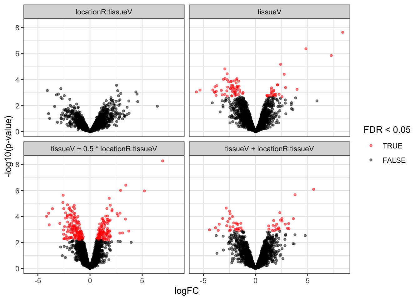

7.7.7 Heatmaps

We use a nominal FDR level of 0.05

alpha <- 0.05

We conduct heatmaps for the significant metabolites for each contrast.

1. We first extract the assay proteins along with its colData.
2. We make an empty list heatmaps to store the plots.
3. We will loop over the column names of the contrast matrix L
4. We extract the names of the significant features for contrast i
5. We extract the quant data for the significant metabolites
6. We extract annotation
7. We make the heatmap using the quants data. We do not cluster columns (samples) to keep them together according to the design.

We only produce heatmaps for the first three contrasts as no DA proteins were returned for the location x tissue interaction.

heatmaps <- lapply(colnames(L)[1:3],
                   function(contrast, se, alpha)
                   {
                     sig <- rowData(se)[[contrast]] |> 
                       filter(adjPval < alpha) |> 
                       rownames()
                     quants <- t(scale(t(assay(se[sig,]))))
                     colnames(quants) <- paste0(se$location, se$tissue, se$patient)
                     annotations <- columnAnnotation(condition = paste0(se$location, se$tissue))
                     set.seed(1234) ## annotation colours are randomly generated by default
                     return(
                       Heatmap(
                       quants, 
                       name = "log2 intensity",
                       top_annotation = annotations, 
                       column_title = paste0(contrast, " = 0")
                       )
                     )
                   },
                   se = getWithColData(pe, "proteins"),
                   alpha = alpha)

Warning: 'experiments' dropped; see 'drops()'

heatmaps

[[1]]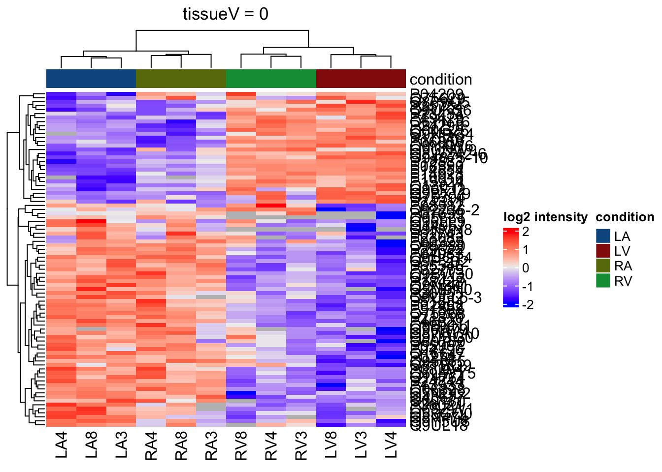

[[2]]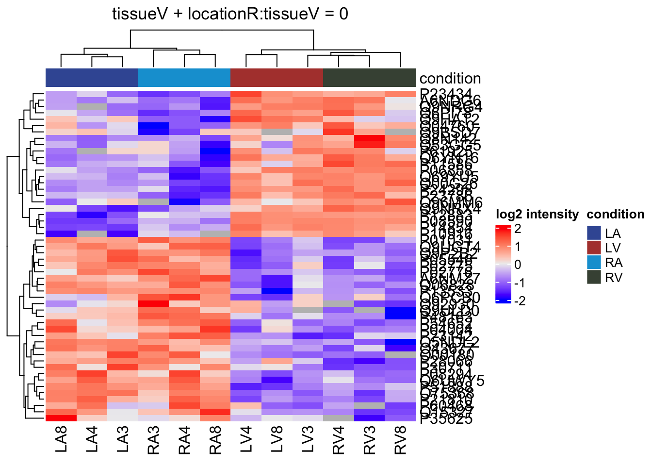

[[3]]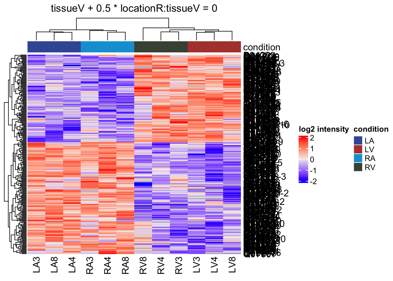

7.8 Conclusion

In this chapter, we illustrated the analysis of a label-free proteomics data set with technical replication. We followed the workflow described in the previous chapters with minimal changes.

The experiment presented in this chapter presents a complex design and is an excellent illustration on how to model data with main effects, interactions and block effects. We could investigate:

1. The difference in protein abundance between the atrium and ventriculum in the left heart compartment.
2. The difference in protein abundance between the atrium and ventriculum in the right heart compartment.
3. The difference in protein abundance between the atrium and ventriculum, averaged over the right and left heart compartment.
4. The interaction, whether the difference between atrium and ventriculum is affected by whether we focus on the left heart or the right heart compartment.

---

1. Note, that upon this transformation a value of 1 represents a p-value of 0.1, 2 a p-value of 0.01, 3 a p-value of 0.001, etc.