1 Statistical analysis with msqrob2 (Data Dependent Acquisition, DDA)
This chapter explains the main concepts for data-processing and statistical analysis of proteomics data using msqrob2. Here, these concepts are introduced using a spike-in study acquired with Data Dependent Acquisition (DDA). The structure, rationale and code of this chapter is very similar to that of the next chapter. The chapters differ primarily in the data importing and filtering steps, which are specific to the respective technologies and search engines. So we refer users who will mainly work with DIA data to chapter 2.
In this chapter, we are using a publicly available spike-in study with PRIDE identifierPXD003881 (Shen et al. 2018). This dataset contains ground truth information about which proteins are differentially abundant, enabling us to objectively demonstrate the key aspects of differential proteomics data analysis and their implementation in msqrob2. This dataset has a relatively simple experimental design (which does not imply that the analysis is easy), allowing us to assess differential abundance using a data analysis workflow with a single factor for the spike-in condition. For more advanced analyses with a more complex experimental design, we refer to our advanced concepts chapter and to the case studies.
1.1 Background
Mass spectrometry (MS)-based proteomics aims at characterising the proteome abundance of biological samples. A popular approach is label-free quantification (LFQ), where every sample is analysed in a separate MS run. This section provides an overview of the analytical workflow and its main challenges regarding data modelling.
1.1.1 LFQ workflow
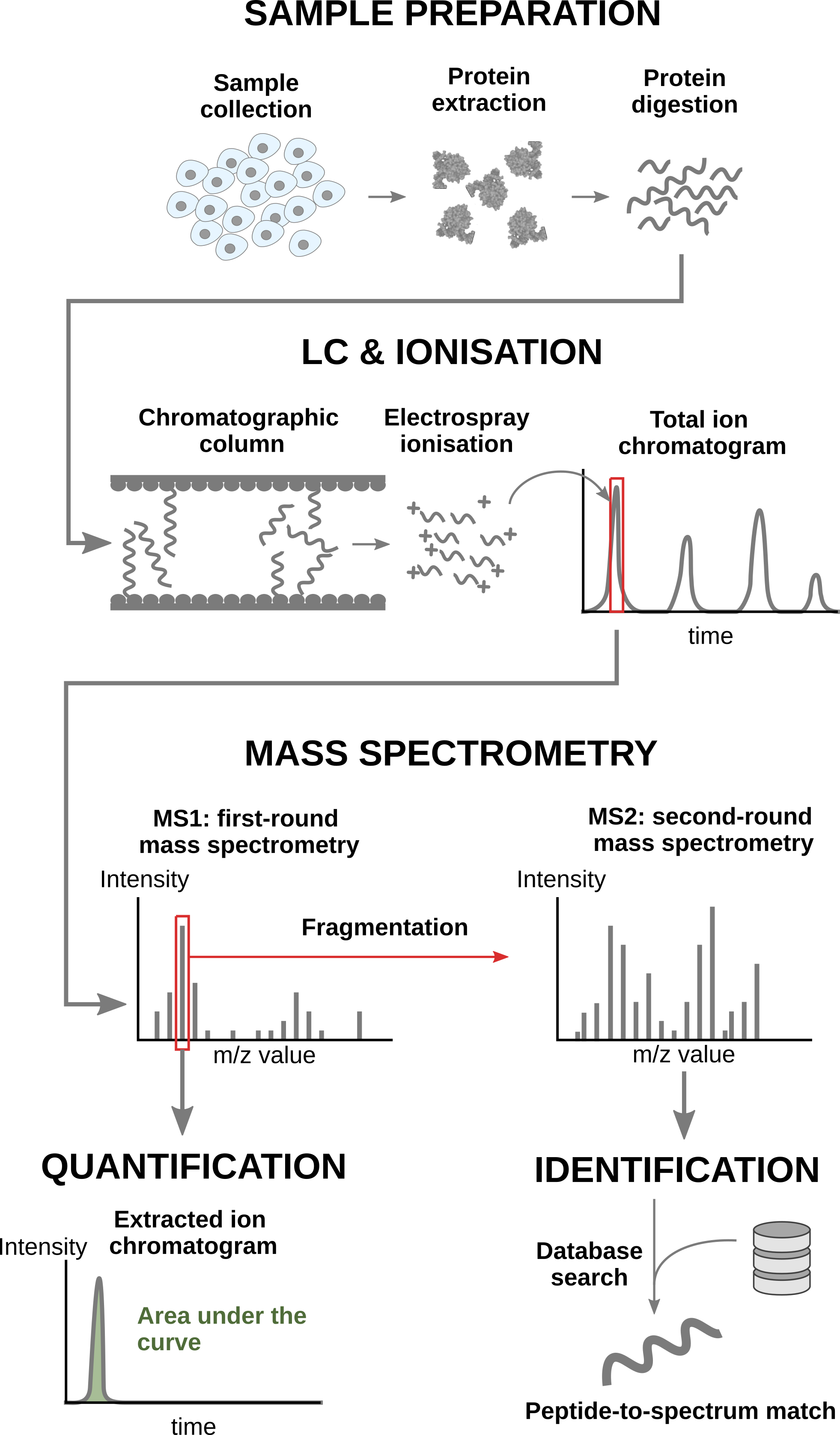
In a nutshell, the wetlab workflow starts with sample preparation where the samples are collected, and the protein content is extracted and digested into peptides. To reduce the sample complexity, the peptides are then separated based on physicochemical properties (mostly hydrophobicity) using liquid chromatography (LC). Peptides are then ionised by an electrospray as they elute from the chromatographic column. The signal over time generated by the eluting ions is called the total ion chromatogram. The ions are then sent for a first round of MS to record their m/z distribution for the intact ions. This provides an overview of the ions that elute from the column and allows for further separation of the ions in the m/z space. The second round of MS (MS2) records the fragmented ions for a selection of ions, generally the most intense MS1 peaks1. This process is repeated for every sample so that every sample is acquired in one MS run. This provides the ion’s mass fingerprint. For LFQ workflows, the accumulated MS1 intensity over time, also known as the area under the curve, around the target mass is used as a quantification measure. On the other hand, the ion mass fingerprint, called the MS2 spectrum, enables computational identification of the corresponding peptide using search engines (e.g. Andromeda has been used for this data set) that will provide peptide-to-spectrum matches (PSM). The quantified PSM are further processed by the software (MaxQuant) to obtain a peptide table2, where every row corresponds to an identified peptide and every column contains information about the peptide and its quantification in one of the samples.
1.1.2 Challenges
Behind this workflow lies several challenges that will affect the data modelling:
- MS-based proteomics does not measure proteins directly, but their constituting peptide ions. The protein-level information needs to be reconstructed from the ion data. In this tutorial, we will start from the peptide data, which has been constructed from the ion data by MaxQuant.
- All peptides do not ionise with the same efficiency. Poor ionisation will lead to reduced signal as less ions will hit the detector, hence leading to a huge variability in intensity among different peptide species, even when they originate from the same protein.
- The identification step is not trivial and prone to errors3. PSM misidentification leads to the assignment of a quantitative values from another peptide with likely another ionisation efficiency and relative abundance. Hence this misassigned values often lead to outliers.
- Moreover, the ion selection for MS2 depends on its intensity4. Therefore, the chance to measure and, subsequently, identify a peptide will depend on its abundance. Non identified peptides will lead to data missingness, which is related to the underlying quantification value. This phenomenon is known as missingness not at random. Next to that, many reasons can lead to ions not being selected or identified irrespective of their quantification value leading to missingness that is not related to its quantitative value. This is referred to as missingness completely at random. The missingness issue is not negligible as we shall see upon reading the data.
- The identification issues lead to unbalanced peptide missingness across samples, and the patterns of missing values are potentially different for every peptide, highlighting the need for an automatised solution that is robust against missing values.
- Technical variations during the experiment can lead to systematic fluctuations across samples. The most obvious reason is when different sample amounts are injected into the instruments, due to small pipetting inconsistencies for instance. However, these differences lead to unwanted variation that should be discarded when answering biological questions.
1.1.3 Experimental context
The samples were synthetically constructed, starting from a trypsin-digested human background, hence human proteins are known to be constant across samples. E. coli lysates were spiked at five different concentrations (3%, 4.5%, 6%, 7.5% and 9% wt/wt). So the E. coli proteins are known to be differentially abundant, and we know exactly in what amount they differ. There are four replicates per spike-in condition. The samples were run on an Orbitrap Fusion mass spectrometer. Raw data files were processed with MaxQuant (version 1.6.1.0) using default search settings unless otherwise noted. Spectra were searched against the UniProtKB/SwissProt human and E. coli reference proteome databases (07/06/2018), concatenated with the default Maxquant contaminant database. Carbamidomethylation of Cystein was set as a fixed modification, and oxidation of Methionine and acetylation of the protein amino-terminus were allowed as variable modifications. In silico cleavage was set to use trypsin/P, allowing two miscleavages. Match between runs was also enabled using default settings. The resulting peptide-to-spectrum matches (PSMs) were filtered by MaxQuant at 1% FDR.
We will start from the peptide data generated by MaxQuant and infer protein-level differences between samples. To achieve this goal, we will apply an msqrob2 workflow, a data processing and modelling workflow dedicated to the analysis of MS-based proteomics datasets. We will demonstrate how the workflow can retrieve the spiked-in proteins from the E. coli data set, while introducing the key statistical concepts of differential proteomics data analysis. Before delving into the analysis, we first set the concentrations for the different spike-ins, and will prepare our computational environment.
concentrations <- (2:6) * 1.5
names(concentrations) <- letters[1:5]
1.2 Software
1.2.1 Load packages
We load the msqrob2 package, along with additional packages for data manipulation and visualisation.
suppressPackageStartupMessages({
library("msqrob2")
library("dplyr")
library("ggplot2")
library("patchwork")
library("tidyr")
})
1.2.2 Parallelisation
msqrob2 can parallelise computations during the model estimation to improve speed. However, we will disable parallelisation to ensure this vignette can be run regardless of hardware. Parallelisation is controlled using the BiocParallel package.
library("BiocParallel")
register(SerialParam())
If you want to use msqrob2 with parallelisation enabled and using 4 cores, you can run the following:
register(MulticoreParam(workers = 4))Be mindful that, while parallelisation can improve speed, it will also consume more RAM because part of the data will be copied multiple times over your different workers. If you experience crashes because you exceeded the amount of available RAM on your machine, you should reduce the number of requested workers.
1.3 Data
The data were reanalysed by Sticker et al. (2020) using MaxQuant and deposited on GitHub. We here retrieve MaxQuant’s peptides.txt for the E. coli study.
library("BiocFileCache")Loading required package: dbplyr
Attaching package: 'dbplyr'The following objects are masked from 'package:dplyr':
ident, sqlbfc <- BiocFileCache()
peptideFile <- bfcrpath(bfc,"https://github.com/statOmics/msqrob2data/raw/refs/heads/main/dda/shen/peptides.txt")Peptide table
Each row in the peptide data table contains information about one peptide (the table below shows the first 6 rows). The columns contains various descriptors about the peptide, such as its sequence, its charge, the amino acid composition, etc. Some of these columns (those starting with Intensity.) contain the quantification values for each sample. The table format where the quantitative values for each sample are contained in a separate column is depicted as the “wide format”, as opposed to the “long format” (eg, the [PSM table]).
We will import the data using the fread function of the data.table package. We set the check.names argument equal to TRUE so that all column names are retrieved using the $ operator. This will result in a replacement of spaces in the column names with a .. We also use argument integer64 = “double” because readQFeatures from the QFeatures package does not process 64-bit integers correctly.
peptides <- data.table::fread(peptideFile, check.names = TRUE, integer64 = "double")
quantCols <- grep("Intensity[.]", names(peptides), value = TRUE)| Sequence | N.term.cleavage.window | C.term.cleavage.window | Amino.acid.before | First.amino.acid | Second.amino.acid | Second.last.amino.acid | Last.amino.acid | Amino.acid.after | A.Count | R.Count | N.Count | D.Count | C.Count | Q.Count | E.Count | G.Count | H.Count | I.Count | L.Count | K.Count | M.Count | F.Count | P.Count | S.Count | T.Count | W.Count | Y.Count | V.Count | U.Count | O.Count | Length | Missed.cleavages | Mass | Proteins | Leading.razor.protein | Start.position | End.position | Gene.names | Protein.names | Unique..Groups. | Unique..Proteins. | Charges | PEP | Score | Identification.type.a1 | Identification.type.a2 | Identification.type.a3 | Identification.type.a4 | Identification.type.b1 | Identification.type.b2 | Identification.type.b3 | Identification.type.b4 | Identification.type.c1 | Identification.type.c2 | Identification.type.c3 | Identification.type.c4 | Identification.type.d1 | Identification.type.d2 | Identification.type.d3 | Identification.type.d4 | Identification.type.e1 | Identification.type.e2 | Identification.type.e3 | Identification.type.e4 | Experiment.a1 | Experiment.a2 | Experiment.a3 | Experiment.a4 | Experiment.b1 | Experiment.b2 | Experiment.b3 | Experiment.b4 | Experiment.c1 | Experiment.c2 | Experiment.c3 | Experiment.c4 | Experiment.d1 | Experiment.d2 | Experiment.d3 | Experiment.d4 | Experiment.e1 | Experiment.e2 | Experiment.e3 | Experiment.e4 | Intensity | Intensity.a1 | Intensity.a2 | Intensity.a3 | Intensity.a4 | Intensity.b1 | Intensity.b2 | Intensity.b3 | Intensity.b4 | Intensity.c1 | Intensity.c2 | Intensity.c3 | Intensity.c4 | Intensity.d1 | Intensity.d2 | Intensity.d3 | Intensity.d4 | Intensity.e1 | Intensity.e2 | Intensity.e3 | Intensity.e4 | Reverse | Potential.contaminant | id | Protein.group.IDs | Mod..peptide.IDs | Evidence.IDs | MS.MS.IDs | Best.MS.MS | Oxidation..M..site.IDs | MS.MS.Count | LFQ.intensity.a1 | LFQ.intensity.a2 | LFQ.intensity.a3 | LFQ.intensity.a4 | LFQ.intensity.b1 | LFQ.intensity.b2 | LFQ.intensity.b3 | LFQ.intensity.b4 | LFQ.intensity.c1 | LFQ.intensity.c2 | LFQ.intensity.c3 | LFQ.intensity.c4 | LFQ.intensity.d1 | LFQ.intensity.d2 | LFQ.intensity.d3 | LFQ.intensity.d4 | LFQ.intensity.e1 | LFQ.intensity.e2 | LFQ.intensity.e3 | LFQ.intensity.e4 |
|---|---|---|---|---|---|---|---|---|---|---|---|---|---|---|---|---|---|---|---|---|---|---|---|---|---|---|---|---|---|---|---|---|---|---|---|---|---|---|---|---|---|---|---|---|---|---|---|---|---|---|---|---|---|---|---|---|---|---|---|---|---|---|---|---|---|---|---|---|---|---|---|---|---|---|---|---|---|---|---|---|---|---|---|---|---|---|---|---|---|---|---|---|---|---|---|---|---|---|---|---|---|---|---|---|---|---|---|---|---|---|---|---|---|---|---|---|---|---|---|---|---|---|---|---|---|---|---|---|---|---|---|---|---|---|---|
| AAAAAAAAAAAAAAAGAGAGAK | QSRFQVDLVSENAGRAAAAAAAAAAAAAAA | AAAAAAAAGAGAGAKQTPADGEASGESEPA | R | A | A | A | K | Q | 18 | 0 | 0 | 0 | 0 | 0 | 0 | 3 | 0 | 0 | 0 | 1 | 0 | 0 | 0 | 0 | 0 | 0 | 0 | 0 | 0 | 0 | 22 | 0 | 1595.8380 | P55011 | P55011 | 93 | 114 | SLC12A2 | Solute carrier family 12 member 2 | yes | yes | 2;3 | 0.00e+00 | 98.407 | By matching | By MS/MS | By MS/MS | By MS/MS | By MS/MS | By matching | By matching | By matching | 1 | NA | NA | NA | NA | NA | NA | 1 | 1 | 1 | NA | 1 | NA | 1 | 1 | NA | NA | NA | 1 | NA | 39754000 | 6378300 | 0 | 0 | 0 | 0 | 0 | 0 | 0 | 4268500 | 7099400 | 0 | 0 | 0 | 8563700 | 6597000 | 0 | 0 | 0 | 6846700 | 0 | 0 | 2115 | 0 | 0;1;2;3;4;5;6;7 | 0;1;2;3 | 2 | 2 | 5715600 | 0 | 0 | 0 | 0 | 0 | 0 | 0 | 4324900 | 8047900 | 0 | 0 | 0 | 9420400 | 5673000 | 0 | 0 | 0 | 5761500 | 0 | |||||||||||||||
| AAAAAAAAAAGAAGGR | ______________________________ | AAAAAAAAAGAAGGRGSGPGRRRHLVPGAG | M | A | A | G | R | G | 12 | 1 | 0 | 0 | 0 | 0 | 0 | 3 | 0 | 0 | 0 | 0 | 0 | 0 | 0 | 0 | 0 | 0 | 0 | 0 | 0 | 0 | 16 | 0 | 1197.6214 | Q86U42 | Q86U42 | 2 | 17 | PABPN1 | Polyadenylate-binding protein 2 | yes | yes | 2 | 0.00e+00 | 275.000 | By MS/MS | By MS/MS | By MS/MS | By MS/MS | By matching | By MS/MS | By MS/MS | By MS/MS | By MS/MS | By MS/MS | By MS/MS | By matching | By MS/MS | By MS/MS | By MS/MS | By MS/MS | By MS/MS | By MS/MS | 1 | 1 | 1 | 1 | 1 | 1 | 1 | 1 | NA | 1 | 1 | 1 | 1 | 1 | 1 | 1 | 1 | NA | 1 | 1 | 1211200000 | 76718000 | 53670000 | 86511000 | 79070000 | 57211000 | 56593000 | 81544000 | 79032000 | 0 | 46087000 | 62303000 | 73292000 | 60707000 | 50560000 | 75644000 | 75246000 | 52106000 | 0 | 74366000 | 70540000 | 1 | 3262 | 1 | 8;9;10;11;12;13;14;15;16;17;18;19;20;21;22;23;24;25 | 4;5;6;7;8;9;10;11;12;13;14;15;16;17;18;19 | 9 | 15 | 68748000 | 59998000 | 74863000 | 70216000 | 57211000 | 63173000 | 69374000 | 69165000 | 0 | 52244000 | 66990000 | 62028000 | 62554000 | 55618000 | 65050000 | 63171000 | 55715000 | 0 | 62578000 | 58656000 | |||||
| AAAAAAALQAK | TILRQARNHKLRVDKAAAAAAALQAKSDEK | RVDKAAAAAAALQAKSDEKAAVAGKKPVVG | K | A | A | A | K | S | 8 | 0 | 0 | 0 | 0 | 1 | 0 | 0 | 0 | 0 | 1 | 1 | 0 | 0 | 0 | 0 | 0 | 0 | 0 | 0 | 0 | 0 | 11 | 0 | 955.5451 | P36578 | P36578 | 354 | 364 | RPL4 | 60S ribosomal protein L4 | yes | yes | 2 | 1.00e-07 | 182.680 | By MS/MS | By MS/MS | By MS/MS | By MS/MS | By MS/MS | By MS/MS | By MS/MS | By MS/MS | By MS/MS | By MS/MS | By MS/MS | By MS/MS | By MS/MS | By MS/MS | By MS/MS | By MS/MS | By MS/MS | By MS/MS | By MS/MS | By MS/MS | 2 | 3 | 4 | 2 | 3 | 2 | 2 | 2 | 3 | 3 | 3 | 2 | 3 | 2 | 3 | 2 | 2 | 3 | 3 | 2 | 1829100000 | 129520000 | 56753000 | 114890000 | 126100000 | 33394000 | 66695000 | 93968000 | 125070000 | 84220000 | 83186000 | 102980000 | 108620000 | 72544000 | 76384000 | 100270000 | 118790000 | 67553000 | 52009000 | 115880000 | 100300000 | 2 | 1762 | 2 | 26;27;28;29;30;31;32;33;34;35;36;37;38;39;40;41;42;43;44;45;46;47;48;49;50;51;52;53;54;55;56;57;58;59;60;61;62;63;64;65;66;67;68;69;70;71;72;73;74;75;76 | 20;21;22;23;24;25;26;27;28;29;30;31;32;33;34;35;36;37;38;39;40;41;42;43;44;45;46;47;48;49;50;51;52;53;54;55;56;57 | 29 | 30 | 116060000 | 63444000 | 99420000 | 111980000 | 33394000 | 74449000 | 79944000 | 109450000 | 85332000 | 94299000 | 110730000 | 91926000 | 74751000 | 84026000 | 86223000 | 99722000 | 72233000 | 56151000 | 97516000 | 83401000 | |||
| AAAAAAGAASGLPGPVAQGLK | ______________________________ | GAASGLPGPVAQGLKEALVDTLTGILSPVQ | M | A | A | L | K | E | 9 | 0 | 0 | 0 | 0 | 1 | 0 | 4 | 0 | 0 | 2 | 1 | 0 | 0 | 2 | 1 | 0 | 0 | 0 | 1 | 0 | 0 | 21 | 0 | 1747.9581 | Q96P70 | Q96P70 | 2 | 22 | IPO9 | Importin-9 | yes | yes | 2;3 | 0.00e+00 | 202.440 | By MS/MS | By MS/MS | By MS/MS | By MS/MS | By MS/MS | By MS/MS | By MS/MS | By MS/MS | By MS/MS | By MS/MS | By MS/MS | By MS/MS | By MS/MS | By MS/MS | By MS/MS | By MS/MS | By MS/MS | By MS/MS | By MS/MS | By MS/MS | 2 | 2 | 2 | 2 | 2 | 2 | 2 | 2 | 2 | 2 | 2 | 2 | 2 | 2 | 2 | 2 | 2 | 2 | 2 | 2 | 1789100000 | 109030000 | 72676000 | 101320000 | 97545000 | 77269000 | 79290000 | 110840000 | 110060000 | 75937000 | 74675000 | 68192000 | 102570000 | 93726000 | 72743000 | 108550000 | 98519000 | 70725000 | 80125000 | 93910000 | 91423000 | 3 | 3783 | 3 | 77;78;79;80;81;82;83;84;85;86;87;88;89;90;91;92;93;94;95;96;97;98;99;100;101;102;103;104;105;106;107;108;109;110;111;112;113;114;115;116 | 58;59;60;61;62;63;64;65;66;67;68;69;70;71;72;73;74;75;76;77;78;79;80;81;82;83;84;85;86;87;88;89;90;91;92;93;94;95;96;97;98;99;100;101;102;103;104;105;106;107 | 85 | 50 | 97706000 | 81244000 | 87682000 | 86622000 | 77269000 | 88508000 | 94294000 | 96324000 | 76939000 | 84650000 | 73322000 | 86806000 | 96578000 | 80020000 | 93344000 | 82709000 | 75624000 | 86506000 | 79024000 | 76020000 | |||
| AAAAAAGAGPEMVR | ______________________________ | MAAAAAAGAGPEMVRGQVFDVGPRYTNLSY | M | A | A | V | R | G | 7 | 1 | 0 | 0 | 0 | 0 | 1 | 2 | 0 | 0 | 0 | 0 | 1 | 0 | 1 | 0 | 0 | 0 | 0 | 1 | 0 | 0 | 14 | 0 | 1241.6187 | P28482 | P28482 | 2 | 15 | MAPK1 | Mitogen-activated protein kinase 1 | yes | yes | 2 | 0.00e+00 | 168.740 | By MS/MS | By MS/MS | By MS/MS | By MS/MS | By MS/MS | By MS/MS | By MS/MS | By MS/MS | By MS/MS | By MS/MS | 1 | 1 | 1 | 1 | NA | 1 | 1 | 1 | NA | 2 | 1 | 1 | NA | NA | NA | NA | NA | NA | NA | NA | 72178000 | 0 | 29646000 | 41064000 | 0 | 0 | 0 | 0 | 0 | 0 | 1468400 | 0 | 0 | 0 | 0 | 0 | 0 | 0 | 0 | 0 | 0 | 4 | 1600 | 4 | 117;118;119;120;121;122;123;124;125;126;127 | 108;109;110;111;112;113;114;115;116;117 | 109 | 10 | 0 | 33141000 | 35535000 | 0 | 0 | 0 | 0 | 0 | 0 | 1664500 | 0 | 0 | 0 | 0 | 0 | 0 | 0 | 0 | 0 | 0 | |||||||||||||
| AAAAAAGSGTPREEEGPAGEAAASQPQAPTSVPGAR | ______________________________ | AASQPQAPTSVPGARLSRLPLARVKALVKA | M | A | A | A | R | L | 12 | 2 | 0 | 0 | 0 | 2 | 4 | 5 | 0 | 0 | 0 | 0 | 0 | 0 | 5 | 3 | 2 | 0 | 0 | 1 | 0 | 0 | 36 | 1 | 3287.5767 | Q9NR33 | Q9NR33 | 2 | 37 | POLE4 | DNA polymerase epsilon subunit 4 | yes | yes | 3 | 3.34e-05 | 40.328 | By MS/MS | NA | NA | NA | NA | NA | NA | NA | NA | NA | NA | NA | 1 | NA | NA | NA | NA | NA | NA | NA | NA | 6961000 | 0 | 0 | 0 | 0 | 0 | 0 | 0 | 0 | 0 | 0 | 0 | 6961000 | 0 | 0 | 0 | 0 | 0 | 0 | 0 | 0 | 5 | 4289 | 5 | 128 | 118 | 118 | 1 | 0 | 0 | 0 | 0 | 0 | 0 | 0 | 0 | 0 | 0 | 0 | 5891200 | 0 | 0 | 0 | 0 | 0 | 0 | 0 | 0 |
Sample annotation table
Each row in the annotation table contains information about one sample. The columns contain various descriptors about the sample, such as the name of the sample or the MS run, the treatment (here the spike-in condition), or any other biological or technical information that may impact the data quality or the quantification. Without an annotation table, no analysis can be performed. The sample annotations are generated by the researcher. In this example, the annotations are extracted from the sample names, although reporting a detailed design of experiments in a table is seen as better practice (Gatto et al. 2023).
coldata <- data.frame(quantCols = quantCols) |>
  mutate(sampleId = gsub("Intensity.(..)", "\\1", quantCols),
         condition = gsub("Intensity.(.).", "\\1", quantCols),
         concentration = concentrations[condition]
)| quantCols | sampleId | condition | concentration |
|---|---|---|---|
| Intensity.a1 | a1 | a | 3.0 |
| Intensity.a2 | a2 | a | 3.0 |
| Intensity.a3 | a3 | a | 3.0 |
| Intensity.a4 | a4 | a | 3.0 |
| Intensity.b1 | b1 | b | 4.5 |
| Intensity.b2 | b2 | b | 4.5 |
We will also extract the E. coli protein identifiers from the FASTA file to later annotate the spike-in proteins which are known to be differentially abundant.
- We download the fasta files
- We read the text file as vector, one line p
- We keep only the protein headers
- We extract the proteins identifiers from the headers
ecoli <- bfcrpath(bfc, "https://github.com/statOmics/msqrob2data/raw/refs/heads/main/dda/shen/ecoli_up000000625_7_06_2018.fasta")
ecoli <- readLines(ecoli)
ecoli <- ecoli[grepl("^>", ecoli)]
ecoli <- gsub(">sp\\|(.*)\\|.*", "\\1", ecoli)
1.3.1 Convert to QFeatures
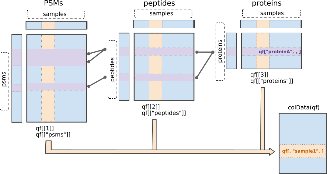
msqrob2 is built around the QFeatures class. We refer to the R for mass spectrometry book for a comprehensive description of the class. In a nutshell, the QFeatures package provides infrastructure to manage and analyse quantitative features from mass spectrometry experiments. It is based on the SummarizedExperiment and MultiAssayExperiment classes. It leverages the hierarchical structure of proteomics experiments: data proteins are composed of peptides, themselves produced by spectra. Each piece of information in stored in an individual SummarizedExperiment object, later referred to as a “set”. Throughout the aggregation and processing of these data, the relations between sets are tracked and recorded, thus allowing users to easily navigate across spectra, peptide and protein quantitative data.
QFeatures data class.The readQFeatures() enables a seamless conversion of tabular data into a QFeatures object. We provide the peptide table and the sample annotation table. The function will use the quantCols column in the sample annotation table to understand which columns in peptides contain the quantitative values, and automatically link the corresponding sample annotation with the quantitative values. We also tell the function to use the Sequence column as peptide identifier, which will be used as rownames. See ?readQFeatures() for more details.
(spikein <- QFeatures::readQFeatures(
  peptides, coldata, name = "peptides", fnames = "Sequence"
))
Checking arguments.Loading data as a 'SummarizedExperiment' object.Formatting sample annotations (colData).Formatting data as a 'QFeatures' object.Setting assay rownames.An instance of class QFeatures (type: bulk) with 1 set:
[1] peptides: SummarizedExperiment with 32827 rows and 20 columns We now have a QFeatures object with 1 set, called peptides (which we specified using the name argument). In this toy example, we have information for 32827 peptides across 45 samples, as expected (recall the experimental design).
The sample annotations can be retrieved using colData().
colData(spikein)knitr::kable(head(colData(spikein)))| quantCols | sampleId | condition | concentration | |
|---|---|---|---|---|
| Intensity.a1 | Intensity.a1 | a1 | a | 3.0 |
| Intensity.a2 | Intensity.a2 | a2 | a | 3.0 |
| Intensity.a3 | Intensity.a3 | a3 | a | 3.0 |
| Intensity.a4 | Intensity.a4 | a4 | a | 3.0 |
| Intensity.b1 | Intensity.b1 | b1 | b | 4.5 |
| Intensity.b2 | Intensity.b2 | b2 | b | 4.5 |
We can get a sample annotation directly using the $ accessor.
head(spikein$concentration) a a a a b b
3.0 3.0 3.0 3.0 4.5 4.5 We can extract the SummarizedExperiment object for the peptides set using double bracket subsetting5
spikein[["peptides"]]class: SummarizedExperiment
dim: 32827 20
metadata(0):
assays(1): ''
rownames(32827): AAAAAAAAAAAAAAAGAGAGAK AAAAAAAAAAGAAGGR ...
YYVTIIDAPGHRDFIK YYYIPQYK
rowData names(116): Sequence N.term.cleavage.window ...
LFQ.intensity.e3 LFQ.intensity.e4
colnames(20): Intensity.a1 Intensity.a2 ... Intensity.e3 Intensity.e4
colData names(0):But notice that the sample annotations were not extracted along with the SummarizedExperiment (colData names(0):). This can be performed using getWithColData(), which extracts the set of interest (like [[]]) along with all the associated sample annotations.
getWithColData(spikein, "peptides")class: SummarizedExperiment
dim: 32827 20
metadata(0):
assays(1): ''
rownames(32827): AAAAAAAAAAAAAAAGAGAGAK AAAAAAAAAAGAAGGR ...
YYVTIIDAPGHRDFIK YYYIPQYK
rowData names(116): Sequence N.term.cleavage.window ...
LFQ.intensity.e3 LFQ.intensity.e4
colnames(20): Intensity.a1 Intensity.a2 ... Intensity.e3 Intensity.e4
colData names(4): quantCols sampleId condition concentrationThe peptides annotations are available for in the corresponding rowData.
rowData(spikein[["peptides"]])knitr::kable(head(rowData(spikein[["peptides"]])))| Sequence | N.term.cleavage.window | C.term.cleavage.window | Amino.acid.before | First.amino.acid | Second.amino.acid | Second.last.amino.acid | Last.amino.acid | Amino.acid.after | A.Count | R.Count | N.Count | D.Count | C.Count | Q.Count | E.Count | G.Count | H.Count | I.Count | L.Count | K.Count | M.Count | F.Count | P.Count | S.Count | T.Count | W.Count | Y.Count | V.Count | U.Count | O.Count | Length | Missed.cleavages | Mass | Proteins | Leading.razor.protein | Start.position | End.position | Gene.names | Protein.names | Unique..Groups. | Unique..Proteins. | Charges | PEP | Score | Identification.type.a1 | Identification.type.a2 | Identification.type.a3 | Identification.type.a4 | Identification.type.b1 | Identification.type.b2 | Identification.type.b3 | Identification.type.b4 | Identification.type.c1 | Identification.type.c2 | Identification.type.c3 | Identification.type.c4 | Identification.type.d1 | Identification.type.d2 | Identification.type.d3 | Identification.type.d4 | Identification.type.e1 | Identification.type.e2 | Identification.type.e3 | Identification.type.e4 | Experiment.a1 | Experiment.a2 | Experiment.a3 | Experiment.a4 | Experiment.b1 | Experiment.b2 | Experiment.b3 | Experiment.b4 | Experiment.c1 | Experiment.c2 | Experiment.c3 | Experiment.c4 | Experiment.d1 | Experiment.d2 | Experiment.d3 | Experiment.d4 | Experiment.e1 | Experiment.e2 | Experiment.e3 | Experiment.e4 | Intensity | Reverse | Potential.contaminant | id | Protein.group.IDs | Mod..peptide.IDs | Evidence.IDs | MS.MS.IDs | Best.MS.MS | Oxidation..M..site.IDs | MS.MS.Count | LFQ.intensity.a1 | LFQ.intensity.a2 | LFQ.intensity.a3 | LFQ.intensity.a4 | LFQ.intensity.b1 | LFQ.intensity.b2 | LFQ.intensity.b3 | LFQ.intensity.b4 | LFQ.intensity.c1 | LFQ.intensity.c2 | LFQ.intensity.c3 | LFQ.intensity.c4 | LFQ.intensity.d1 | LFQ.intensity.d2 | LFQ.intensity.d3 | LFQ.intensity.d4 | LFQ.intensity.e1 | LFQ.intensity.e2 | LFQ.intensity.e3 | LFQ.intensity.e4 | |
|---|---|---|---|---|---|---|---|---|---|---|---|---|---|---|---|---|---|---|---|---|---|---|---|---|---|---|---|---|---|---|---|---|---|---|---|---|---|---|---|---|---|---|---|---|---|---|---|---|---|---|---|---|---|---|---|---|---|---|---|---|---|---|---|---|---|---|---|---|---|---|---|---|---|---|---|---|---|---|---|---|---|---|---|---|---|---|---|---|---|---|---|---|---|---|---|---|---|---|---|---|---|---|---|---|---|---|---|---|---|---|---|---|---|---|---|---|
| AAAAAAAAAAAAAAAGAGAGAK | AAAAAAAAAAAAAAAGAGAGAK | QSRFQVDLVSENAGRAAAAAAAAAAAAAAA | AAAAAAAAGAGAGAKQTPADGEASGESEPA | R | A | A | A | K | Q | 18 | 0 | 0 | 0 | 0 | 0 | 0 | 3 | 0 | 0 | 0 | 1 | 0 | 0 | 0 | 0 | 0 | 0 | 0 | 0 | 0 | 0 | 22 | 0 | 1595.8380 | P55011 | P55011 | 93 | 114 | SLC12A2 | Solute carrier family 12 member 2 | yes | yes | 2;3 | 0.00e+00 | 98.407 | By matching | By MS/MS | By MS/MS | By MS/MS | By MS/MS | By matching | By matching | By matching | 1 | NA | NA | NA | NA | NA | NA | 1 | 1 | 1 | NA | 1 | NA | 1 | 1 | NA | NA | NA | 1 | NA | 39754000 | 0 | 2115 | 0 | 0;1;2;3;4;5;6;7 | 0;1;2;3 | 2 | 2 | 5715600 | 0 | 0 | 0 | 0 | 0 | 0 | 0 | 4324900 | 8047900 | 0 | 0 | 0 | 9420400 | 5673000 | 0 | 0 | 0 | 5761500 | 0 | |||||||||||||||
| AAAAAAAAAAGAAGGR | AAAAAAAAAAGAAGGR | ______________________________ | AAAAAAAAAGAAGGRGSGPGRRRHLVPGAG | M | A | A | G | R | G | 12 | 1 | 0 | 0 | 0 | 0 | 0 | 3 | 0 | 0 | 0 | 0 | 0 | 0 | 0 | 0 | 0 | 0 | 0 | 0 | 0 | 0 | 16 | 0 | 1197.6214 | Q86U42 | Q86U42 | 2 | 17 | PABPN1 | Polyadenylate-binding protein 2 | yes | yes | 2 | 0.00e+00 | 275.000 | By MS/MS | By MS/MS | By MS/MS | By MS/MS | By matching | By MS/MS | By MS/MS | By MS/MS | By MS/MS | By MS/MS | By MS/MS | By matching | By MS/MS | By MS/MS | By MS/MS | By MS/MS | By MS/MS | By MS/MS | 1 | 1 | 1 | 1 | 1 | 1 | 1 | 1 | NA | 1 | 1 | 1 | 1 | 1 | 1 | 1 | 1 | NA | 1 | 1 | 1211200000 | 1 | 3262 | 1 | 8;9;10;11;12;13;14;15;16;17;18;19;20;21;22;23;24;25 | 4;5;6;7;8;9;10;11;12;13;14;15;16;17;18;19 | 9 | 15 | 68748000 | 59998000 | 74863000 | 70216000 | 57211000 | 63173000 | 69374000 | 69165000 | 0 | 52244000 | 66990000 | 62028000 | 62554000 | 55618000 | 65050000 | 63171000 | 55715000 | 0 | 62578000 | 58656000 | |||||
| AAAAAAALQAK | AAAAAAALQAK | TILRQARNHKLRVDKAAAAAAALQAKSDEK | RVDKAAAAAAALQAKSDEKAAVAGKKPVVG | K | A | A | A | K | S | 8 | 0 | 0 | 0 | 0 | 1 | 0 | 0 | 0 | 0 | 1 | 1 | 0 | 0 | 0 | 0 | 0 | 0 | 0 | 0 | 0 | 0 | 11 | 0 | 955.5451 | P36578 | P36578 | 354 | 364 | RPL4 | 60S ribosomal protein L4 | yes | yes | 2 | 1.00e-07 | 182.680 | By MS/MS | By MS/MS | By MS/MS | By MS/MS | By MS/MS | By MS/MS | By MS/MS | By MS/MS | By MS/MS | By MS/MS | By MS/MS | By MS/MS | By MS/MS | By MS/MS | By MS/MS | By MS/MS | By MS/MS | By MS/MS | By MS/MS | By MS/MS | 2 | 3 | 4 | 2 | 3 | 2 | 2 | 2 | 3 | 3 | 3 | 2 | 3 | 2 | 3 | 2 | 2 | 3 | 3 | 2 | 1829100000 | 2 | 1762 | 2 | 26;27;28;29;30;31;32;33;34;35;36;37;38;39;40;41;42;43;44;45;46;47;48;49;50;51;52;53;54;55;56;57;58;59;60;61;62;63;64;65;66;67;68;69;70;71;72;73;74;75;76 | 20;21;22;23;24;25;26;27;28;29;30;31;32;33;34;35;36;37;38;39;40;41;42;43;44;45;46;47;48;49;50;51;52;53;54;55;56;57 | 29 | 30 | 116060000 | 63444000 | 99420000 | 111980000 | 33394000 | 74449000 | 79944000 | 109450000 | 85332000 | 94299000 | 110730000 | 91926000 | 74751000 | 84026000 | 86223000 | 99722000 | 72233000 | 56151000 | 97516000 | 83401000 | |||
| AAAAAAGAASGLPGPVAQGLK | AAAAAAGAASGLPGPVAQGLK | ______________________________ | GAASGLPGPVAQGLKEALVDTLTGILSPVQ | M | A | A | L | K | E | 9 | 0 | 0 | 0 | 0 | 1 | 0 | 4 | 0 | 0 | 2 | 1 | 0 | 0 | 2 | 1 | 0 | 0 | 0 | 1 | 0 | 0 | 21 | 0 | 1747.9581 | Q96P70 | Q96P70 | 2 | 22 | IPO9 | Importin-9 | yes | yes | 2;3 | 0.00e+00 | 202.440 | By MS/MS | By MS/MS | By MS/MS | By MS/MS | By MS/MS | By MS/MS | By MS/MS | By MS/MS | By MS/MS | By MS/MS | By MS/MS | By MS/MS | By MS/MS | By MS/MS | By MS/MS | By MS/MS | By MS/MS | By MS/MS | By MS/MS | By MS/MS | 2 | 2 | 2 | 2 | 2 | 2 | 2 | 2 | 2 | 2 | 2 | 2 | 2 | 2 | 2 | 2 | 2 | 2 | 2 | 2 | 1789100000 | 3 | 3783 | 3 | 77;78;79;80;81;82;83;84;85;86;87;88;89;90;91;92;93;94;95;96;97;98;99;100;101;102;103;104;105;106;107;108;109;110;111;112;113;114;115;116 | 58;59;60;61;62;63;64;65;66;67;68;69;70;71;72;73;74;75;76;77;78;79;80;81;82;83;84;85;86;87;88;89;90;91;92;93;94;95;96;97;98;99;100;101;102;103;104;105;106;107 | 85 | 50 | 97706000 | 81244000 | 87682000 | 86622000 | 77269000 | 88508000 | 94294000 | 96324000 | 76939000 | 84650000 | 73322000 | 86806000 | 96578000 | 80020000 | 93344000 | 82709000 | 75624000 | 86506000 | 79024000 | 76020000 | |||
| AAAAAAGAGPEMVR | AAAAAAGAGPEMVR | ______________________________ | MAAAAAAGAGPEMVRGQVFDVGPRYTNLSY | M | A | A | V | R | G | 7 | 1 | 0 | 0 | 0 | 0 | 1 | 2 | 0 | 0 | 0 | 0 | 1 | 0 | 1 | 0 | 0 | 0 | 0 | 1 | 0 | 0 | 14 | 0 | 1241.6187 | P28482 | P28482 | 2 | 15 | MAPK1 | Mitogen-activated protein kinase 1 | yes | yes | 2 | 0.00e+00 | 168.740 | By MS/MS | By MS/MS | By MS/MS | By MS/MS | By MS/MS | By MS/MS | By MS/MS | By MS/MS | By MS/MS | By MS/MS | 1 | 1 | 1 | 1 | NA | 1 | 1 | 1 | NA | 2 | 1 | 1 | NA | NA | NA | NA | NA | NA | NA | NA | 72178000 | 4 | 1600 | 4 | 117;118;119;120;121;122;123;124;125;126;127 | 108;109;110;111;112;113;114;115;116;117 | 109 | 10 | 0 | 33141000 | 35535000 | 0 | 0 | 0 | 0 | 0 | 0 | 1664500 | 0 | 0 | 0 | 0 | 0 | 0 | 0 | 0 | 0 | 0 | |||||||||||||
| AAAAAAGSGTPREEEGPAGEAAASQPQAPTSVPGAR | AAAAAAGSGTPREEEGPAGEAAASQPQAPTSVPGAR | ______________________________ | AASQPQAPTSVPGARLSRLPLARVKALVKA | M | A | A | A | R | L | 12 | 2 | 0 | 0 | 0 | 2 | 4 | 5 | 0 | 0 | 0 | 0 | 0 | 0 | 5 | 3 | 2 | 0 | 0 | 1 | 0 | 0 | 36 | 1 | 3287.5767 | Q9NR33 | Q9NR33 | 2 | 37 | POLE4 | DNA polymerase epsilon subunit 4 | yes | yes | 3 | 3.34e-05 | 40.328 | By MS/MS | NA | NA | NA | NA | NA | NA | NA | NA | NA | NA | NA | 1 | NA | NA | NA | NA | NA | NA | NA | NA | 6961000 | 5 | 4289 | 5 | 128 | 118 | 118 | 1 | 0 | 0 | 0 | 0 | 0 | 0 | 0 | 0 | 0 | 0 | 0 | 5891200 | 0 | 0 | 0 | 0 | 0 | 0 | 0 | 0 |
We can also retrieve the quantitative values for each set using assays(). Here we only show the first 5 rows and columns of the intensity matrix.
assay(spikein[[1]])[1:5, 1:5] Intensity.a1 Intensity.a2 Intensity.a3 Intensity.a4
AAAAAAAAAAAAAAAGAGAGAK 6378300 0 0 0
AAAAAAAAAAGAAGGR 76718000 53670000 86511000 79070000
AAAAAAALQAK 129520000 56753000 114890000 126100000
AAAAAAGAASGLPGPVAQGLK 109030000 72676000 101320000 97545000
AAAAAAGAGPEMVR 0 29646000 41064000 0
Intensity.b1
AAAAAAAAAAAAAAAGAGAGAK 0
AAAAAAAAAAGAAGGR 57211000
AAAAAAALQAK 33394000
AAAAAAGAASGLPGPVAQGLK 77269000
AAAAAAGAGPEMVR 01.4 Data preprocessing
Since we have a QFeatures object, we can directly make use of QFeatures’ data preprocessing functionality6. A major advantage of QFeatures is it provides the power to build highly modular workflows, where each step is carried out by a dedicated function with a large choice of available methods and parameters. This means that users can adapt the workflow to their specific use case and their specific needs.
1.4.1 Encoding missing values
The first preprocessing step is to correctly encode the missing values. It is important that missing values are encoded using NA. For instance, non-observed values should not be encoded with a zero because true zeros (the proteomic feature is absent from the sample) cannot be distinguished from technical zeros (the feature was missed by the instrument or could not be identified). We therefore replace any zero in the quantitative data with an NA.
spikein <- zeroIsNA(spikein, names(spikein))Note that msqrob2 can handle missing data without having to rely on hard-to-verify imputation assumptions, which is our general recommendation. However, msqrob2 does not prevent users from using imputation, which can be performed with impute() from the QFeatures package. Below, we show how one could perform KNN imputation7 (see ?impute for more options).
# spikein <- impute(
#   spikein, method = "knn",
#   i = names(spikein), name = paste0(names(spikein), "_imput")
# )
1.4.2 Log2 transformation
We typically start a MS-based proteomics data analysis by log2 transforming the intensities. We illustrate the rationale using the spike-in data. For this, we perform a short data manipulation pipeline:
- We use
longForm()to convert theQFeaturesobject into a long table, where each row contains the quantitative information about one observation, in which column, row and set it was found. Long tables are particularly useful for manipulating data with thetidyverseecosystem, namely withggplot2for visualisation.longForm()also allows to include annotations, and we here includeMixtureandTechRepMixturefor filtering and colouring. longForm()returns aDataFramewhich we convert to adata.frame.- We filter the data to keep only the data from peptide AEMSEYLFDK.
dat <- longForm(spikein, colvars = colnames(colData(spikein))) |> ## 1.
  data.frame() |> ## 2.
  filter(rowname == "AEMSEYLFDK") ## 3.
Next, we visualise the data using ggplot2. We will show the intensities and log2-intensities for one of the peptides, AALEELVK, in function of the known E. coli spike-in concentration. We first define a common plot from which we generate two plots, one without and the other with log2 transformation of the quantitative values.
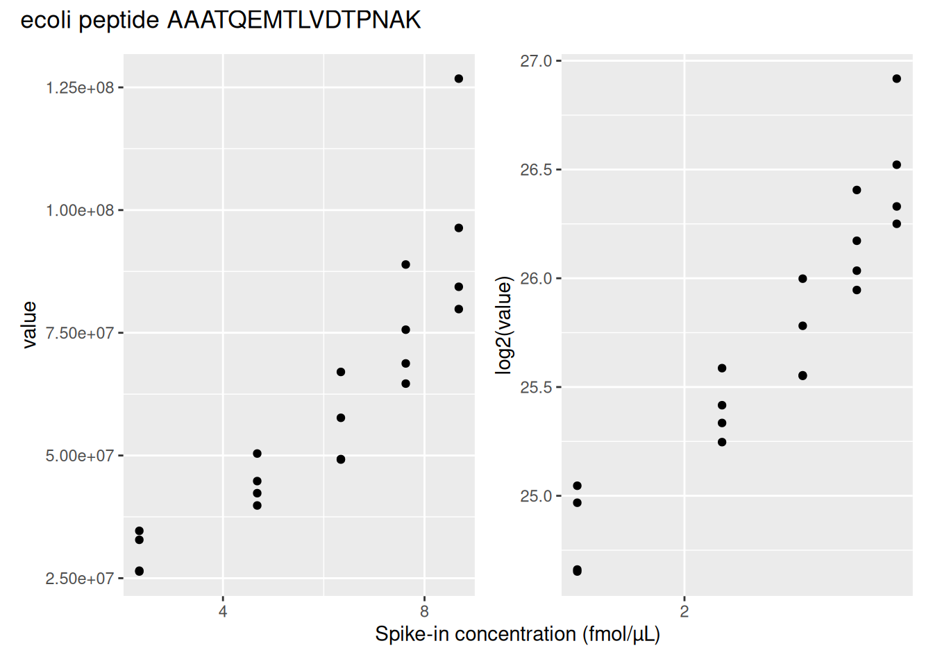
We can see that the variation around the mean for each concentration slightly increases as the mean increases. This is known as heteroskedasticity. We will later see that msqrob2 assumes that variance of the error is equal across the different conditions. Upon, log2-transformation we can see that the problem of unequal variability is solved.
Another advantages of log2-transformation is that it provides a scale that directly relates to biological interpretation. In biology, a change induced by some condition often results in a fold change in concentration. Interestingly, the log2 fold change (logFC), which is the log2 of the ratio between two conditions, is identical to the difference between the log of each condition.
\[log_2FC_{b-a} = log_2b - log_2a = log_2 \frac{b}{a}\]
This simplifies the modelling since the effects are now additive and it provides a straightforward interpretation, i.e. a logFC of 1 means that the abundances are on average \(2\times\) higher in \(b\) than in \(a\), a logFC of 2 means an average increase of \(4\times\), for instance. Also, note that the averages calculated at the log2-scale have the interpretation of log2-transformed geometric means.
We perform log2-transformation with logTransform() from the QFeatures package.
spikein <- logTransform(
  spikein, "peptides", name = "peptides_log", base = 2
)
1.4.3 Peptide filtering
Filtering removes low-quality and unreliable peptides that would otherwise introduce noise and artefacts in the data. There are many possible criteria for peptide filtering:
- Reverse sequences
- Only identified by modification site (only modified peptides detected)
- Razor peptides: non-unique peptides assigned to the protein group with the most other peptides
- Contaminants
- Peptides with few identifications
- Proteins that are only identified with one or a few peptides
- FDR of identification
- …
It is important that the filtering criteria are not distorting the distribution of the test statistics in the downstream analysis for features that are non-DA. It can be shown that filtering will not induce bias results when the filtering criterion is independent of test statistic. Here, the test statistics are based on the average difference between the log2-transformed intensities (effect size) and their corresponding standard error, which is a function of the residual standard deviation. The criteria that we proposed above are all based on the results of the identification step, hence, they are independent of the downstream test statistics that will be used to prioritize DA proteins.
We use filterFeatures() to perform the filtering. It uses information from the rowData and a formula to generate a filter for each feature (row) in each set across the object. If the filter returns TRUE, the corresponding row is retained, otherwise it is removed. Defining a filter through a formula offers a flexible approach, allowing for any customised filter. This dataset requires an extensive PSM filtering, which is an ideal use case to demonstrate the customisation of a filtering workflow.
Remove failed protein inference
We remove peptides that could not be mapped to a protein. We also remove peptides that cannot be uniquely mapped to a single proteins because its sequence is shared across multiple proteins. This often occurs for homologs or for proteins that share similar functional domains. Shared peptides are often mapped to protein groups, which are the set of proteins that share the given peptides. Protein groups are encoded by appending the constituting protein identifiers, separated by a ";".
spikein <- filterFeatures(
  spikein, ~ Proteins != "" & ## Remove failed protein inference
    !grepl(";", Proteins)) ## Remove protein groups
'Proteins' found in 2 out of 2 assay(s).Remove reverse sequences and contaminants
We now remove the peptides that map to decoy sequences or to contaminants proteins. Decoy peptides, which consist of fake peptide sequences generated by reversing a real amino-acid sequence, are used during the database search to mitigating the number of random-hit PSM, hence mitigating misidentification. Contaminant proteins are proteins known to be artificially incorporated during the experiment, but that are irrelevant to the biological system under study. Typical contaminants are human or animal keratins (deposited by the experimenter) or trypsin (used for protein digestion). It is important to remove these peptides before performing statistical modelling, otherwise these proteins will be accounted for during the multiple test adjustment, which will cause an unnecessary decrease of statistical power. Note, that the column name of the contaminants in the peptides file differs according to the MaxQuant version. In our peptide.txt file decoys and contaminants are indicated with a “+” character in the column Reverse and Potential.contaminant, respectively.
spikein <- filterFeatures(spikein, ~ Reverse != "+" & ## Remove decoys
                            Potential.contaminant != "+") ## Remove contaminants
'Reverse' found in 2 out of 2 assay(s).'Potential.contaminant' found in 2 out of 2 assay(s).Remove highly missing peptides
The data are characterised by a high proportion of missing values as reported by nNA() from the QFeatures package. The function computes the number and the proportion of missing values across peptides, samples or for the whole data set and return a list of three tables called nNArows, nNAcols, and nNA, respectively.
nNaRes <- nNA(spikein, "peptides")
range(nNaRes$nNAcols$pNA)
[1] 0.2196928 0.2649294The samples contain between 22% and 26.5% missing values. The missingness within each peptide is more variable, with most peptides found accross all samples (nNA is 0) and other that could not be quantified in any sample (nNA is 20), as depicted by the histogram below.
data.frame(nNaRes$nNArows) |>
  ggplot() +
  aes(x = nNA) +
  geom_histogram(bins = 15) +
  ggtitle("Number of missing values for each peptide") +
  theme_bw()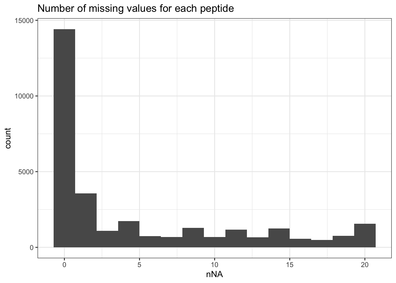
We keep peptides that were observed at last 4 times out of the \(n = 20\) samples, so that we can estimate the peptide characteristics. We tolerate the following proportion of NAs: \(\text{pNA} = \frac{(n - 4)}{n} = 0.8\), so we keep peptides that are observed in at least 20% of the samples, which corresponds to one treatment condition. This is an arbitrary value that may need to be adjusted depending on the experiment and the data set.
nObs <- 4
n <- ncol(spikein[["peptides_log"]])
(spikein <- filterNA(spikein, i = "peptides_log", pNA = (n - nObs) / n))
An instance of class QFeatures (type: bulk) with 2 sets:
[1] peptides: SummarizedExperiment with 30661 rows and 20 columns
[2] peptides_log: SummarizedExperiment with 27850 rows and 20 columns We keep 27850 peptides upon filtering.
1.4.4 Identifications per sample
spikein[,,"peptides"] |>
  longForm(colvars = colnames(colData(spikein)),
           rowvars= c("Sequence",
                      "Proteins")) |>
  data.frame() |>
  filter(!is.na(value)) |>
  group_by(condition, sampleId) |>
  summarise(peptides = length(unique(Sequence)),
            Proteins = length(unique(Proteins))) |>
  pivot_longer(-(1:2),
               names_to = "Feature",
               values_to = "IDs") |>
  ggplot(aes(x = sampleId, y = IDs, fill = condition)) +
  geom_col() +
  #scale_fill_observable() +
  facet_wrap(~Feature,
             scales = "free_y") +
  labs(title = "Peptide and protein group identificiations per sample",
       x = "Sample",
       y = "Identifications") +
  theme_bw() +
  theme(axis.text.x = element_text(angle = 90))
Warning: 'experiments' dropped; see 'drops()'harmonizing input:
removing 20 sampleMap rows not in names(experiments)`summarise()` has regrouped the output.
ℹ Summaries were computed grouped by condition and sampleId.
ℹ Output is grouped by condition.
ℹ Use `summarise(.groups = "drop_last")` to silence this message.
ℹ Use `summarise(.by = c(condition, sampleId))` for per-operation grouping
(`?dplyr::dplyr_by`) instead.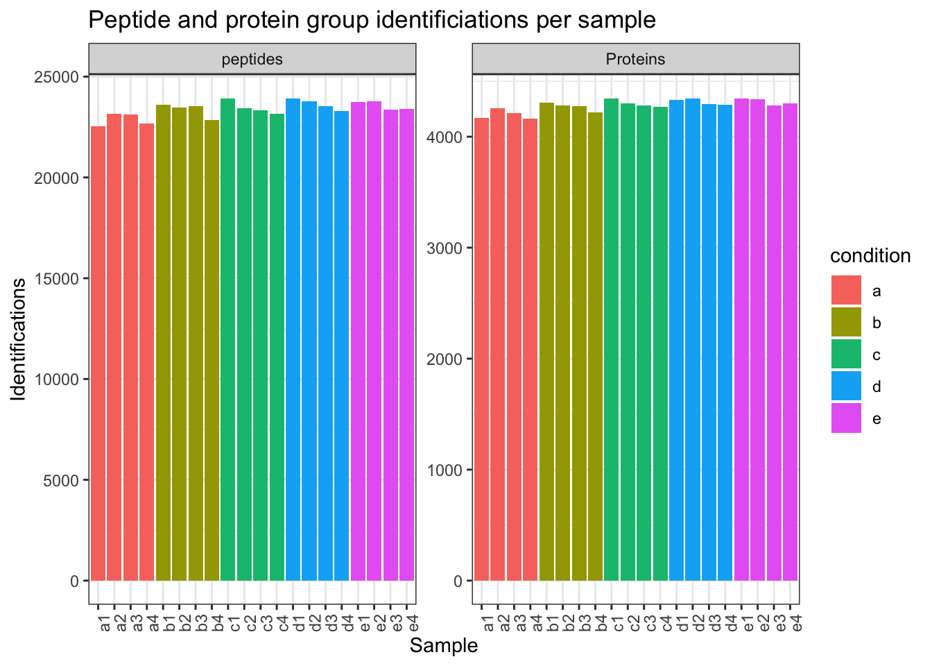
1.4.5 Normalisation
The most common objective of MS-based proteomics experiments is to understand the biological changes in protein abundance between experimental conditions. However, changes in measurements between groups can be caused due to technical factors. For instance, there are systematic fluctuations from run-to-run that shift the measured intensity distribution. We can this explore as follows:
- We extract the sets containing the log transformed data. This is performed using
QFeatures’ 3-way subsetting8. - We use
longForm()to convert theQFeaturesobject into a long table, includingconditionandconcentrationfor filtering and colouring. - We visualise the density of the quantitative values within each sample. We colour each sample based on its spike-in condition.
spikein[, , "peptides_log"] |> ## 1.
  longForm(colvars = c("concentration", "condition")) |> ## 2.
  data.frame() |>
  ggplot() + ## 3.
  aes(x = value,
      colour = condition,
      group = colname) +
  geom_density() +
  theme_bw()
Warning: 'experiments' dropped; see 'drops()'harmonizing input:
removing 20 sampleMap rows not in names(experiments)Warning: Removed 92133 rows containing non-finite outside the scale range
(`stat_density()`).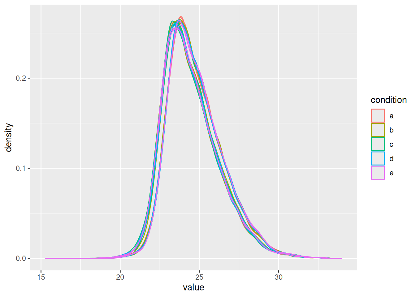
Even in this clean synthetic data set (same background with a small percentage of E. coli lysate), the marginal peptide intensity distributions across samples are not well aligned. Ignoring this effect will increase the noise and reduce the statistical power of the experiment, and may also, in case of unbalanced designs, introduce confounding effects that will bias the results.
Therefore, normalisation will transform the data to make the intensities of the different samples comparable, e.g. by centering the distributions using the median, so that the distributions better coincide and overlap.
Subtracting the sample median at the log scale from each precursor log2 intensity, basically boils down to calculating log-ratio’s between the precursor intensity and its sample median.
Here, we will use the Median of Ratios method of DESeq2, which was originally developed for RNA-seq data analysis and can also correct for differences in composition of the proteomes in the different samples. The method first calculates pseudo-reference sample (row-wise mean of log2 intensities, which corresponds to the log2 transformed geometric mean). THen calculates log2 ratios of each sample w.r.t. the pseudo-reference. Finally the column wise median of these log2 ratios is taken to obtain the sample based normalisation factor on the log2 scale. This procedure is implemented in the msqrob2 function nfLogMedianOfRatios.
- We calculate the log transformed normalisation factor from the Median of Ratios method
- Subtract these log2-norm factors from the intensities of each corresponding column of the assay data and store the result in the new assay peptides_norm. (We adopt the sweep function to the
peptides_logassay of the spikein QFeatures object with as statistic the log2 normfactorSTATS = nfLogthe default functionFUN = "-",MARGIN = 2to substract the column wise log2 norm factor from each entry of the corresponding assay data).
nfLog <- nfLogMedianOfRatios(spikein, "peptides_log") #1.This function aims to calculate norm factors on a log scale,
the input data are assumed to be on the log-scale!spikein <- sweep( #Subtract log2 norm factor column-by-column (MARGIN = 2) #2.
spikein,
MARGIN = 2,
STATS = nfLog,
i = "peptides_log",
name = "peptides_norm"
)Note that users can also use all normalisation functions that are provided in QFeatures, i.e. by replacing the sweep function by QFeatures::normalize.
Formally, the function applies the following operation on each sample \(i\) across all PSMs \(p\):
\[ y_{ip}^{\text{norm}} = y_{ip} - \hat{\mu}_i \]
with \(y_ip\) the log2-transformed intensities and \(\hat{\mu}_i\) the log2-transformed norm factor. Upon normalisation, we can see that the distribution of the \(y_{ip}^{\text{norm}}\) nicely overlap (using the same code as above).
spikein[, , "peptides_norm"] |> ## 1.
  longForm(colvars = c( "concentration", "condition")) |> ## 2.
  data.frame() |>
  ggplot() + ## 3.
  aes(x = value,
      colour = condition,
      group = colname) +
  geom_density()
Warning: 'experiments' dropped; see 'drops()'harmonizing input:
removing 40 sampleMap rows not in names(experiments)Warning: Removed 92133 rows containing non-finite outside the scale range
(`stat_density()`).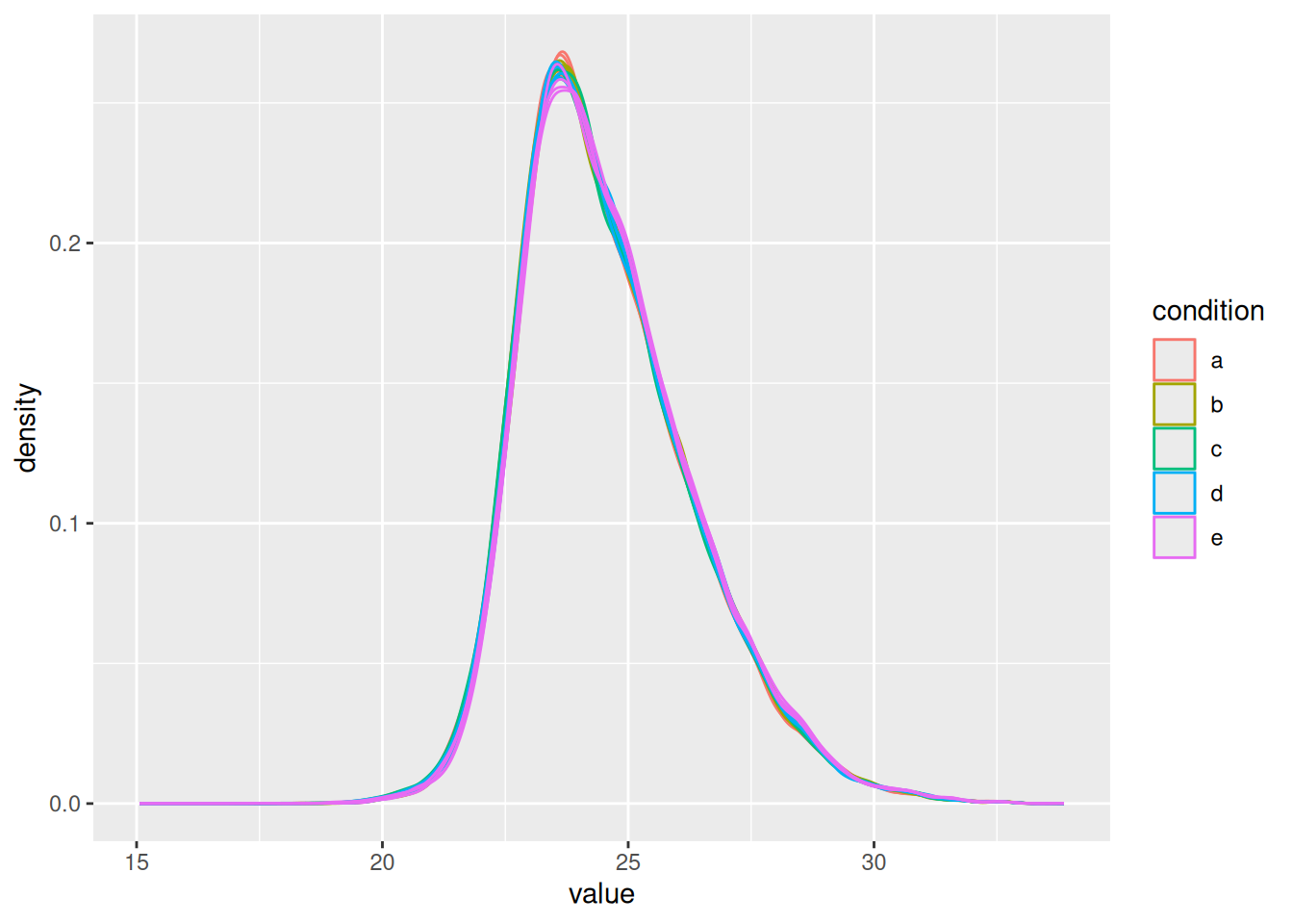
Beware there exist numerous types of normalisation methods (see ?normalize) and which method to use may be data set dependent. For instance, some data set may show low overlap of distribution tails upon normalisation indicating that a simple shift is not sufficient. In micro-array literature, quantile normalisation is used to force the median and all other quantiles to be equal across samples, but in proteomics, quantile normalisation often introduces artifacts due to a difference in missing peptides across samples (c.f. Challenges).
It is important to understand that most normalisation procedures assume that the majority of the proteins do not change across conditions and only a small proportion of the proteins are differentially abundant. This assumption may not be valid in poorly designed spike-in studies (O’Brien et al. 2024) or for pull-down studies, for example. Dedicated normalisation strategies are then required.
1.4.6 Summarisation
The objective of summarisation (also referred to as aggregation) is to summarise the peptide-level intensities into a protein expression value. We illustrate the motivation for summarisation using all peptide-level data for one of the E. coli proteins. We also focus on the lowest (a) and highest (e) spike-in conditions. The different peptides are shown on the x axis and plot their log2 normalised intensities across samples on y axis. All the points belonging to the same sample are linked through a grey line.
Warning: 'experiments' dropped; see 'drops()'harmonizing input:
removing 40 sampleMap rows not in names(experiments)Warning: Removed 20 rows containing missing values or values outside the scale range
(`geom_point()`).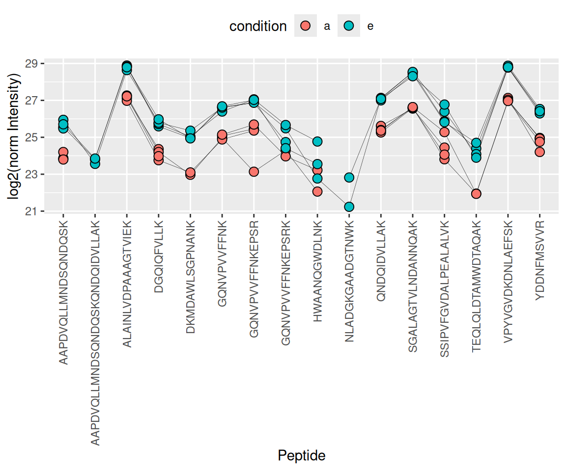
- We can see that data for a protein can consist of many peptides, hence the need for summarisation.
- We observe that different peptides have different intensities within the same sample (same line). This is because different peptides have different properties and hence differ in their ionisation efficiency, which will influence the detectability in the MS (Challenges).
- The peptide identification are inconsistent between groups of interest. We can see the low-concentration group (condition a, red) display more missing values than the high-concentration group (condition e, blue). Moreover, which value is missing depends on the peptide characteristics. All the peptides found in the low-concentration group are the most intense peptides in the high concentration group.
- We also often find outliers, for instance, due to misidentification or fluctuations during MS acquisition.
- These data also suggest pseudo-replication. The peptide intensities in one same sample (dots connected by a line) are correlated, i.e. they more alike than the peptide intensities between samples (the lines do not perfectly align).
The fact that different peptides have different intensities (2.), may be inconsistently identified (3.) and/or quantified (4.), and show sample correlations (5.) can lead to bias if we use simple summarisation approaches such as summing or averaging the peptide intensities for each sample. Instead, we will resort to more advanced summarisation approaches to accommodate for these issues.
Here, we summarise the peptide-level data into protein intensities through the robust summarisation approach (Sticker et al. 2020) which is a model approach that estimates for each protein \(P\) separately:
\[ y_{ip} = \beta_p^\text{pep} + \beta_i^\text{samp} + \epsilon_{ip} \]
where \(y_{ip}\) is the log-normalised peptide intensity for peptide \(p\) belonging to protein \(P\) in sample \(i\). \(\beta_p^\text{pep}\) is the average effect of peptide \(p\), which account for the fact that different peptide yield different baseline intensities (see issue 2. above). \(\beta_i^\text{samp}\) is the average effect of sample \(i\). In other words, it provides the estimated log2-transformed and normalised intensity of protein \(P\) in sample \(i\) corrected for the peptide effect, which will be used as the summarised protein value. \(\epsilon_{ip}\) is the residual effect that cannot be explained by the average sample and peptide effects. The method is called robust summarisation because the estimation process will minimize \(\epsilon\) using a robust estimator9 that will down-weigh extreme values, effectively tackling issue 4.
aggregateFeatures() streamlines summarisation. It requires the name of a rowData column to group the peptides into proteins (or protein groups), here Proteins. We provide the summarisation approach through the fun argument. Other summarisation methods are available from the MsCoreUtils package, see ?aggregateFeatures for a comprehensive list. The function will return a QFeatures object with a new set that we called proteins.
(spikein <- aggregateFeatures(
  spikein, i = "peptides_norm",
  name = "proteins",
  fcol = "Proteins",
  fun = MsCoreUtils::robustSummary,
  na.rm = TRUE
))
Your quantitative and row data contain missing values. Please read the
relevant section(s) in the aggregateFeatures manual page regarding the
effects of missing values on data aggregation.
Aggregated: 1/1An instance of class QFeatures (type: bulk) with 4 sets:
[1] peptides: SummarizedExperiment with 30661 rows and 20 columns
[2] peptides_log: SummarizedExperiment with 27850 rows and 20 columns
[3] peptides_norm: SummarizedExperiment with 27850 rows and 20 columns
[4] proteins: SummarizedExperiment with 4592 rows and 20 columns Note that all the links between peptides and proteins are kept10. This come particularly handy when we want to extract all the data from one protein, P0AEE5 for instance. This can be performed using the 3-way indexing. Every QFeatures object contains one or more sets, each characterised by multiple rows (peptides or proteins) and multiple columns (samples). Therefore, QFeatures can subset data based on one or more of these indices, data[set_k, feature_i, sample_j]. The first entry will subset particular features. This can be the name of a peptide (e.g. DGQIQFVLLK) or the name of a protein (P0AEE5). The second entry selects the samples columns of interest. The third entry selects the sets of interest. If an entry is left blank, all the corresponding features, samples or sets will be selected. Let’s extract all the data (all samples and all sets) related to the E. coli protein (P0AEE5).
spikein["P0AEE5", , ]An instance of class QFeatures (type: bulk) with 4 sets:
[1] peptides: SummarizedExperiment with 16 rows and 20 columns
[2] peptides_log: SummarizedExperiment with 16 rows and 20 columns
[3] peptides_norm: SummarizedExperiment with 16 rows and 20 columns
[4] proteins: SummarizedExperiment with 1 rows and 20 columns The function extracted one protein and its 16 related peptides. This functionality is particularly useful for plotting and exploring the changes induces by the data processing. For instance:
- We use the
QFeaturessubsetting functionality to keep only the data for the E. coli protein P0AEE5 and the sets before and after summarisation. - We use
longForm()to convert the object for plotting. - We plot the intensities for each sample, facetting by set and colouring by experimental condition, linking dots from the same peptide or protein with a line.
spikein["P0AEE5", , c("peptides_norm", "proteins")] |> ## 1.
  longForm(colvars = colnames(colData(spikein))) |> ## 2.
  data.frame() |>
  ggplot() + ## 3.
  aes(x = colname,
      y = value,
      group = rowname) +
  geom_line(linewidth = 0.1) +
  geom_point(aes(colour = condition)) +
  facet_grid(~ assay) +
  theme(axis.text.x = element_blank()) +
  theme_bw()
Warning: 'experiments' dropped; see 'drops()'harmonizing input:
removing 40 sampleMap rows not in names(experiments)Warning: Removed 25 rows containing missing values or values outside the scale range
(`geom_line()`).Warning: Removed 45 rows containing missing values or values outside the scale range
(`geom_point()`).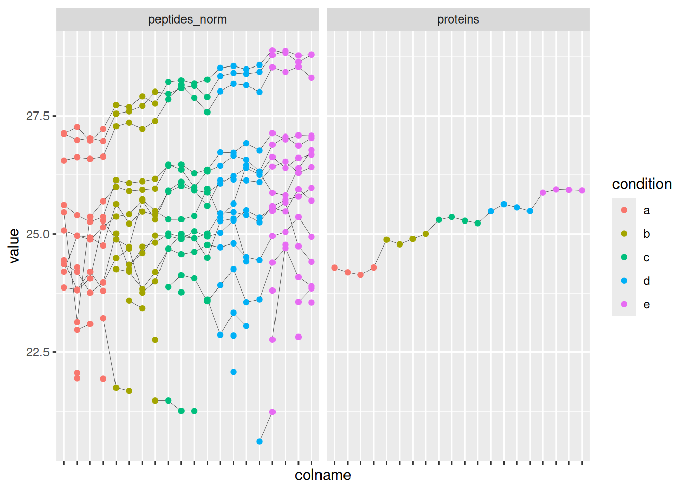
The data processing is complete.
plot(spikein)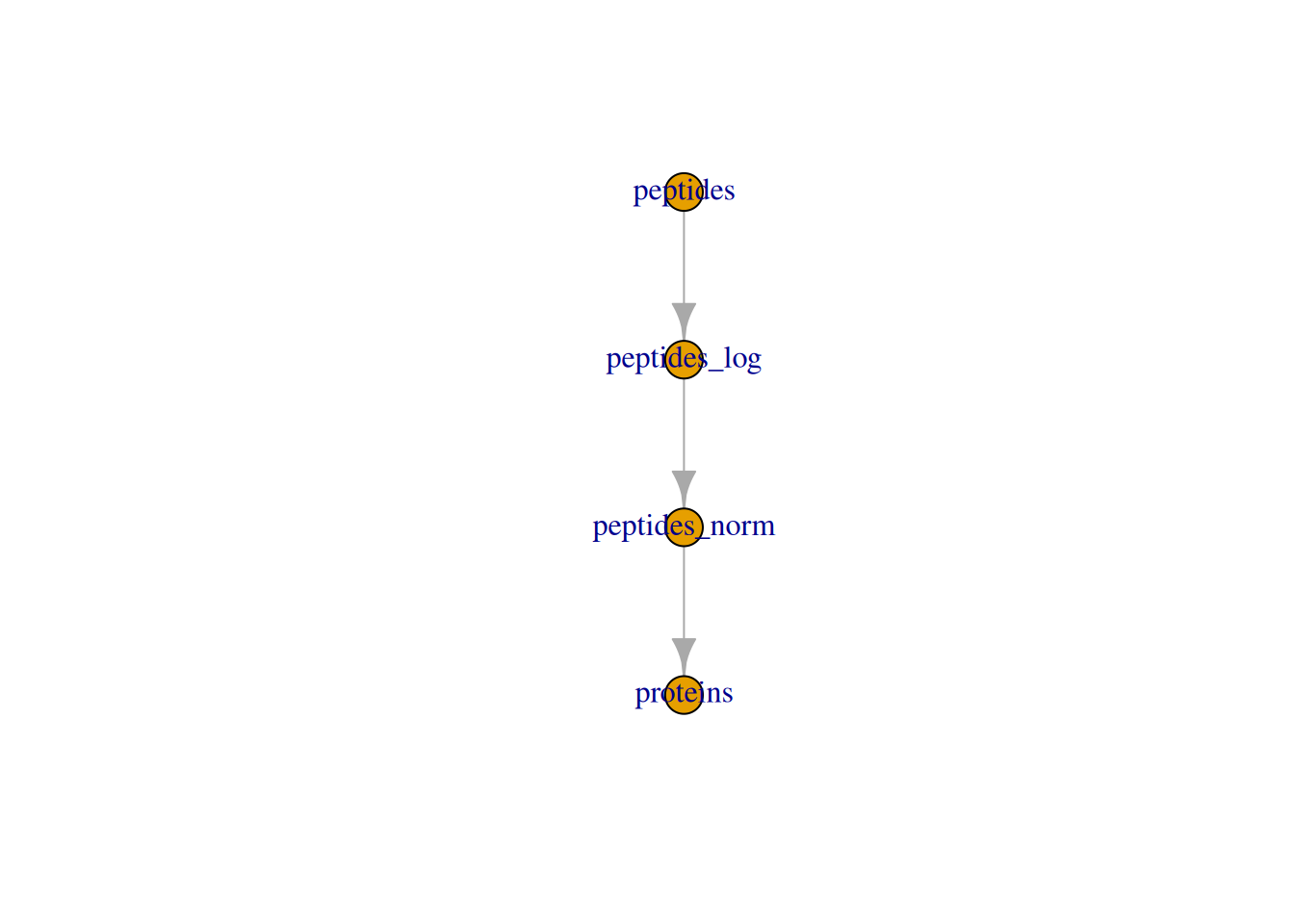
QFeatures object and its processed sets.1.5 Data exploration
Data exploration aims to highlight the main sources of variation in the data prior to data modelling and can pinpoint to outlying or off-behaving samples. A common approach for data exploration is to perform dimension reduction, such as Multi Dimensional Scaling (MDS). We will first extract the set to explore along the sample annotations (used for plot colouring).
se <- getWithColData(spikein, "proteins")Warning: 'experiments' dropped; see 'drops()'We then use the scater package to compute and plot the PCA. For technical reasons, it requires SingleCellExperiment class object, but these can easily be generated from a SummarizedExperiment object.
library("scater")Loading required package: SingleCellExperimentLoading required package: scuttlese <- runMDS(as(se, "SingleCellExperiment"), exprs_values = 1)We can now explore the data structure while coloring for the factor of interest, here condition.
plotMDS(se, colour_by = "condition") 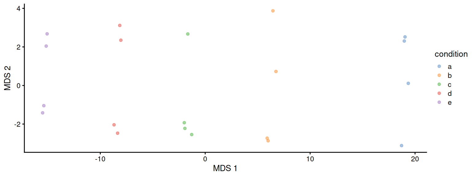
This plot reveals interesting information. First, we see that the samples are nicely separated according to their spike-in condition. Interestingly, the conditions are sorted by the concentration11. We also see some structure in the second dimension. This would probe us to contact the lab where the data were collected to ask if the samples were obtained in batches. It demonstrates the power of data exploration for QC.
1.6 Data modelling
We model the preprocessed data to answer biologically relevant questions. As described above, each sample has been synthetically created to contain a constant human background where E. coli lysates were spiked in at five different concentration. Each sample preparation has been replicated four times. So, the key question is “can our model retrieve the proteins that have been spiked in across the conditions?” Moreover, since we know the expected protein abundance in each sample, we will also be able to assess how accurate the model can estimate the average fold changes between spike-in conditions.
1.6.1 Sources of variation
In this experimental design, we can model a single source of variation: spike-in concentration12. All remaining sources of variability, e.g. pipetting errors, MS run to run variability, etc will be lumped in the residual variability (error term).
Spike-in condition effects: we model the source of variation induced by the experimental treatment of interest as a fixed effect, which we consider non-random, i.e. the treatment effect is assumed to be the same in repeated experiments, but it is unknown and has to be estimated.
When modelling a typical label-free experiment at the protein level, the model boils down to the following linear model:
\[ y_i = \mathbf{x}^T_i \boldsymbol{\beta} + \epsilon_i \]
with \(y_i\) the \(\log_2\)-normalised and summarised protein intensities in sample \(i\); \(\mathbf{x}_i\) a vector with the covariate pattern for the sample encoding the intercept, spike-in condition13, or other experimental factors; \(\boldsymbol{\beta}\) the vector of parameters that model the association between the covariates and the outcome; and \(\epsilon_i\) the residuals reflecting variation that is not captured by the fixed effects. Note that \(\mathbf{x}_i\) allows for a flexible parameterisation of the treatment beyond a single covariate, i.e. including a 1 for the intercept, continuous and categorical variables as well as their interactions. We assume the residuals to be independent and identically distributed (i.i.d) according to a normal distribution with zero mean and constant variance, i.e. \(\epsilon_{i} \sim N(0,\sigma_\epsilon^2)\), that can differ from protein to protein.
In R, this model is encoded using the following simple formula14:
model <- ~ condition1.6.2 Model estimation
We estimate the model with msqrob(). The function takes the QFeatures object, extracts the quantitative values from the "proteins" set generated during summarisation, and fits a simple linear model with condition as covariate, which are automatically retrieved from colData(spikein).
spikein <- msqrob(
  spikein,  i = "proteins",
  formula = model,
  robust = TRUE
)
We enable M-estimation (robust = TRUE) for improved robustness against outliers. We can also enable ridge regression (ridge = TRUE), which can stabilise the parameter estimation of fixed effects. However, this is numerically more complex and is only possible with msqrob2 if there are more than two slope terms in the model, e.g. designs with more than two groups or designs involving multiple covariates. The next chapter provides more details on robust regression and ridge regression.
The fitting results are available in the msqrobModels column of the rowData. More specifically, the modelling output is stored in the rowData as a statModel object, one model per row (protein). We will see in a later section how to perform statistical inference on the estimated parameters.
models <- rowData(spikein[["proteins"]])[["msqrobModels"]]
models[1:3]
$A0AVT1
Object of class "StatModel"
The type is "rlm"
There number of elements is 5
$A0FGR8
Object of class "StatModel"
The type is "rlm"
There number of elements is 5
$A0MZ66
Object of class "StatModel"
The type is "rlm"
There number of elements is 5 1.7 Statistical inference
We can now convert the biological question “does the spike-in condition affect the protein intensities?” into a statistical hypothesis. In other words, we must convert this question in a combination of the model parameters, also referred to as a contrast. To aid defining contrasts, we will visualise the experimental design using the ExploreModelMatrix package.
library("ExploreModelMatrix")
VisualizeDesign(
  sampleData =  colData(spikein),
  designFormula = model,
  textSizeFitted = 4
)$plotlist
[[1]]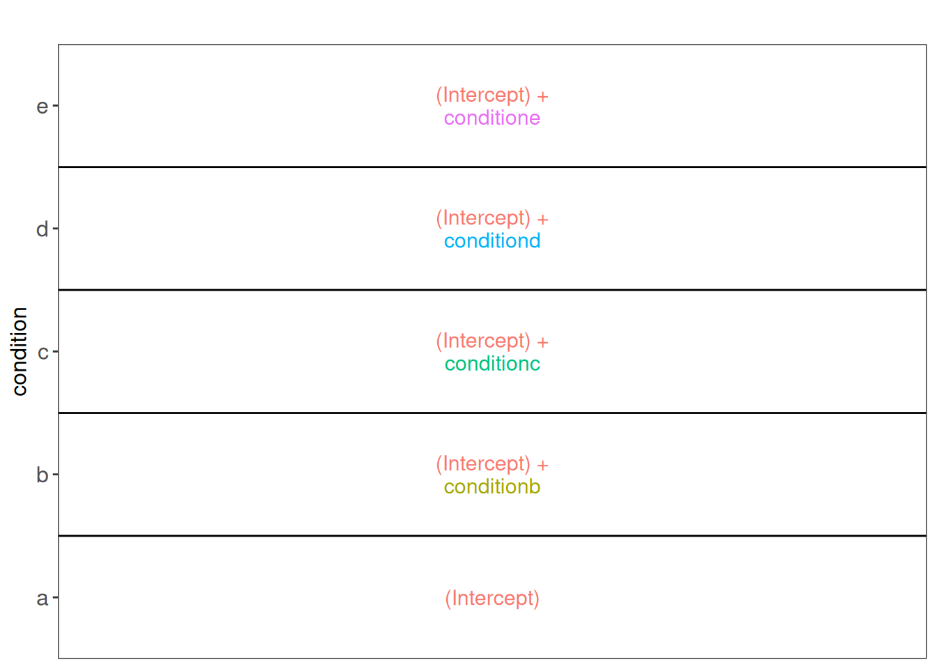
ExploreModelMatrix package.Spike-in condition a is the reference group. So the mean log2 intensity for samples from condition a is (Intercept). The mean log2 expression for samples from condition b is ‘(Intercept) + conditionb’. Hence, the average log2 fold change between condition b and condition a is modelled using the parameter ‘conditionb’.
With getCoef(), we can retrieve the estimated model parameters. We start with extracting the model output, stored as StatModel objects, from the rowData. Next, getCoef() retrieves the estimated model parameters:
models <- rowData(spikein[["proteins"]])$msqrobModels
params <- getCoef(models[[1]])
head(params)
(Intercept) conditionb conditionc conditiond conditione
23.506173482 0.104948589 0.027846447 -0.008119888 -0.071619774 We are interested, for this data set, in the parameters that model the effect of condition.
params[grep("condition", names(params))] conditionb conditionc conditiond conditione
0.104948589 0.027846447 -0.008119888 -0.071619774 For this protein we can see that the effects of condition are small, as expected since the protein is part of the human constant background. We now explore the parameters for one of the E. coli proteins.
params <- getCoef(models[["P0AEE5"]])
params[grep("condition", names(params))]
conditionb conditionc conditiond conditione
0.6625094 1.0662914 1.3155302 1.6919511 Since this is a benchmark study and we know the concentration of A (0.25 fmol/µL) and B (0.74 fmol/µL), the obvious answer is \(log_2(4.5) - log_2(3) = 0.585\). The average log2 difference in intensity between condition B and condition A that has been estimated by the model is 0.6625094, rather close. Now, the question is if we can conclude that the fold change between condition B and condition A is statistically significant for this protein based on the model output.
1.7.1 Hypothesis testing
As shown above, the average difference in log2 intensity between condition b and a after correcting for the lab effect is conditionb. This combination of parameters is also called a contrast. Thus, we assess the following null hypothesis for this contrast: conditionb = 0 with our statistical test.
contrast <- "conditionb = 0"makeContrast() converts the hypothesis into a formal contrast matrix with parameter names as rows and hypotheses in columns15.
(L <- makeContrast(
  "conditionb = 0",
  "conditionb"
))
conditionb
conditionb 1We can now test our null hypothesis using hypothesisTest() which takes the QFeatures object with the fitted model and the contrast we just built. msqrob2 automatically applies the hypothesis testing to all proteins in the data.
spikein <- hypothesisTest(spikein, i = "proteins", contrast = L)The results are stored in the set containing the model, here proteins. We retrieve the results from the rowData. Note, that for this spike-in study we know the ground truth, so we also add variable isEcoli to indicate if the protein is spiked (from E. coli).
#inference <- rowData(spikein[["proteins"]])$ridgeconditionb
inference <- rowData(spikein[["proteins"]])$conditionb
inference$Protein <- rownames(inference)
inference$isEcoli <- inference$Protein %in% ecoli
head(inference)
logFC se df t pval adjPval Protein
A0AVT1 0.10494859 0.07901174 15.963899 1.3282658 0.2027682 0.6845834 A0AVT1
A0FGR8 0.06906717 0.04535794 16.141441 1.5227140 0.1471798 0.5908265 A0FGR8
A0MZ66 -0.10892095 0.06295311 16.313394 -1.7301916 0.1024661 0.4872344 A0MZ66
A1L0T0 -0.02486814 0.18978721 16.791528 -0.1310317 0.8973073 0.9858930 A1L0T0
A1X283 -0.15880954 0.44509882 5.288059 -0.3567962 0.7350432 0.9680034 A1X283
A2RRP1 -0.12957365 0.09296872 14.972800 -1.3937339 0.1837409 0.6617389 A2RRP1
isEcoli
A0AVT1 FALSE
A0FGR8 FALSE
A0MZ66 FALSE
A1L0T0 FALSE
A1X283 FALSE
A2RRP1 FALSENote, that missing values can occur because data modelling resulted in a fitError (the advanced vignette describes how to deal with proteins that could not be fit).
The results also include an adjusted p-value for each protein \(j\) to correct for multiple testing using the Benjamini-Hochberg False Discovery Rate (FDR) method, which represents an estimate of the minimum FDR at which the test result for protein \(j\) is considered significant, i.e. the expected fraction of false positives that are reported in the shortest top list of the most significant proteins that include protein \(j\).
1.7.2 Volcano plots
A volcano plot is a common visualisation that provides an overview of the hypothesis testing results, plotting the \(-\log_{10}\) p-value16 as a function of the estimated log fold change. Volcano plots can be used to highlight the most interesting proteins that have large fold changes and/or are highly significant. We can use the table above directly to build a volcano plot using the plotVolcano function of msqrob2.
inference |>
  plotVolcano() +
  ggtitle("Statistical inference results",
          paste0("H0: ", colnames(L), " = 0"))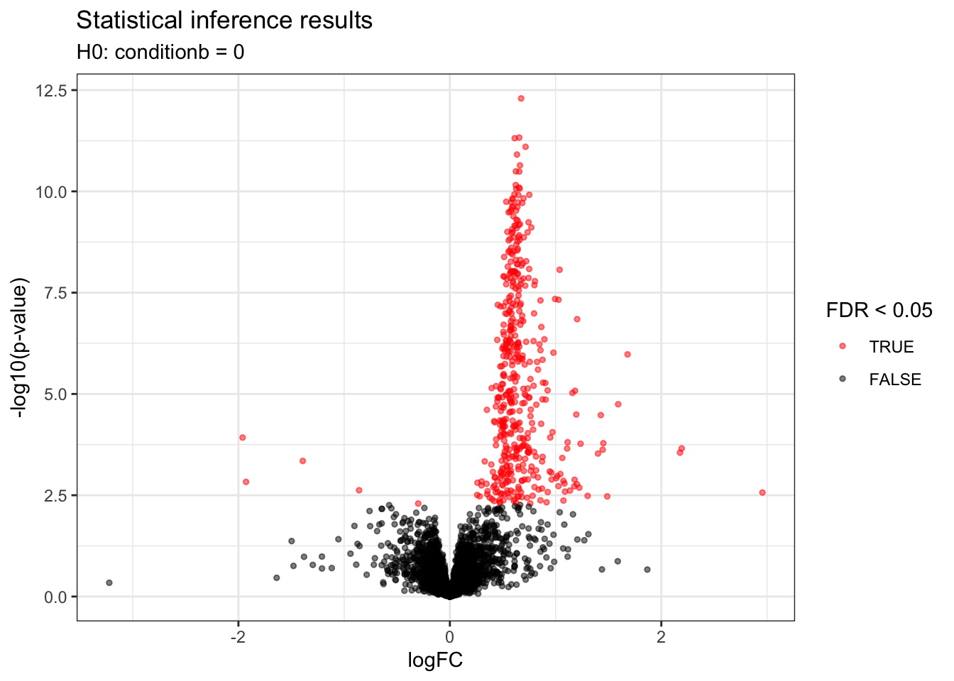
Note, that we also know the ground truth for this dataset because it is a spike-in study. So we will color the dots according to the ground truth in isEcoli and will use a different shape according to the significance (FDR above or below \(\alpha = 0.05\)). We also add a vertical line according to the real logFC.
alpha <- 0.05
inference |>
  plotVolcano() +
  ggtitle("Statistical inference results",
          paste0("H0: ", colnames(L), " = 0")) +
  aes(color = isEcoli, shape = adjPval < alpha) +
    scale_color_manual(
      values = c("grey20", "firebrick"),
      name = "species",
      labels = c("human", "ecoli")
      ) +
  labs(shape = paste0("FDR < ",alpha)) +
  geom_vline(xintercept = log2(4.5) - log2(3), linetype = "dashed")
Scale for colour is already present.
Adding another scale for colour, which will replace the existing scale.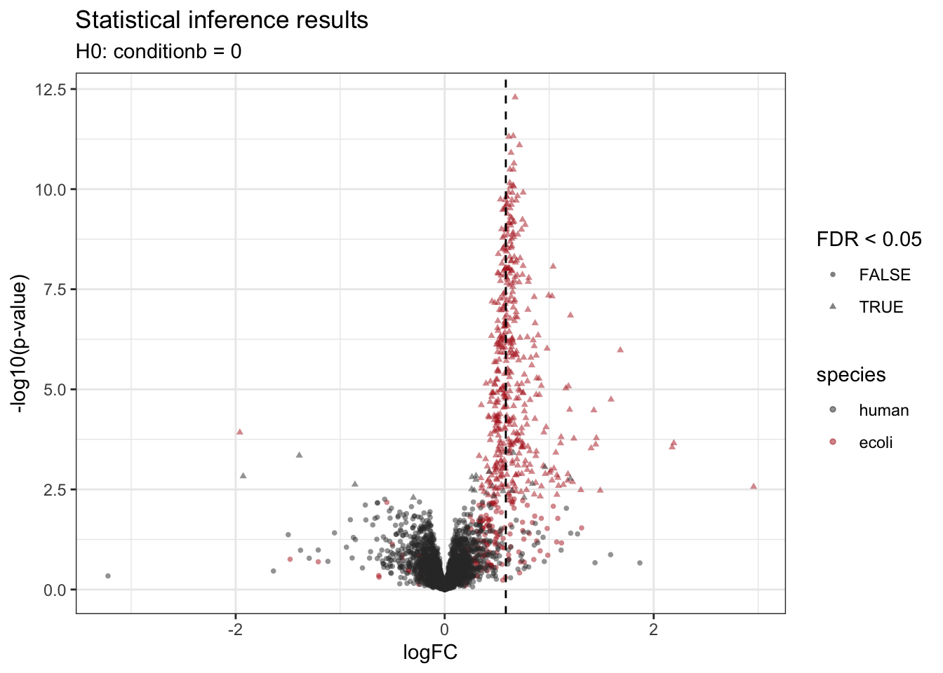
We retrieve the proteins that are significantly differentially abundant based on the FDR-adjusted p-value (adjPval). Note that the majority of the differentially abundant proteins are E. coli proteins.
table(is_significant = inference$adjPval < alpha,
      is_ecoli = inference$isEcoli)
is_ecoli
is_significant FALSE TRUE
FALSE 3716 199
TRUE 21 447Because we known the ground truth, we can also provide a list with false positives, true positives and the false discovery proprotion (FP/(FP+TP)) at a nominal 5% FDR level and observe that the FDP for this contrast is close to the 5% FDR, which is an estimate of the expected FDP if all assumptions made in the data analysis are valid.
inference |>
  filter(adjPval < alpha) |>
  summarise(
    fp = sum(!isEcoli),
    tp = sum(isEcoli),
    fdp = round(mean(!isEcoli) * 100, 2))
fp tp fdp
1 21 447 4.491.7.3 Heatmaps
We can explore the quantitative data of the significant proteins using a heatmap. First, we select the names of the proteins that were declared significant between condition A and condition B and extract their quantitative data.
sigNames <- inference$Protein[!is.na(inference$adjPval) & inference$adjPval < alpha]
se <- getWithColData(spikein, "proteins")
Warning: 'experiments' dropped; see 'drops()'se <- se[sigNames, se$condition %in% c("a", "b")]Next, we extract the quantitative data and scale by rows17 with assay(). We will create a heatmap using the ComplexHeatmap package, which enables heatmap annotations. We will annotate the heatmap using our model variables condition and lab.
quants <- t(scale(t(assay(se))))
library("ComplexHeatmap")
Loading required package: grid========================================
ComplexHeatmap version 2.26.1
Bioconductor page: http://bioconductor.org/packages/ComplexHeatmap/
Github page: https://github.com/jokergoo/ComplexHeatmap
Documentation: http://jokergoo.github.io/ComplexHeatmap-reference
If you use it in published research, please cite either one:
- Gu, Z. Complex Heatmap Visualization. iMeta 2022.
- Gu, Z. Complex heatmaps reveal patterns and correlations in multidimensional
genomic data. Bioinformatics 2016.
The new InteractiveComplexHeatmap package can directly export static
complex heatmaps into an interactive Shiny app with zero effort. Have a try!
This message can be suppressed by:
suppressPackageStartupMessages(library(ComplexHeatmap))
========================================annotations <- columnAnnotation(
condition = se$condition
)We now make the heatmap.
set.seed(1234) ## annotation colours are randomly generated by default
Heatmap(
 quants, name = "log2 intensity",
 cluster_rows = FALSE,
 top_annotation = annotations
)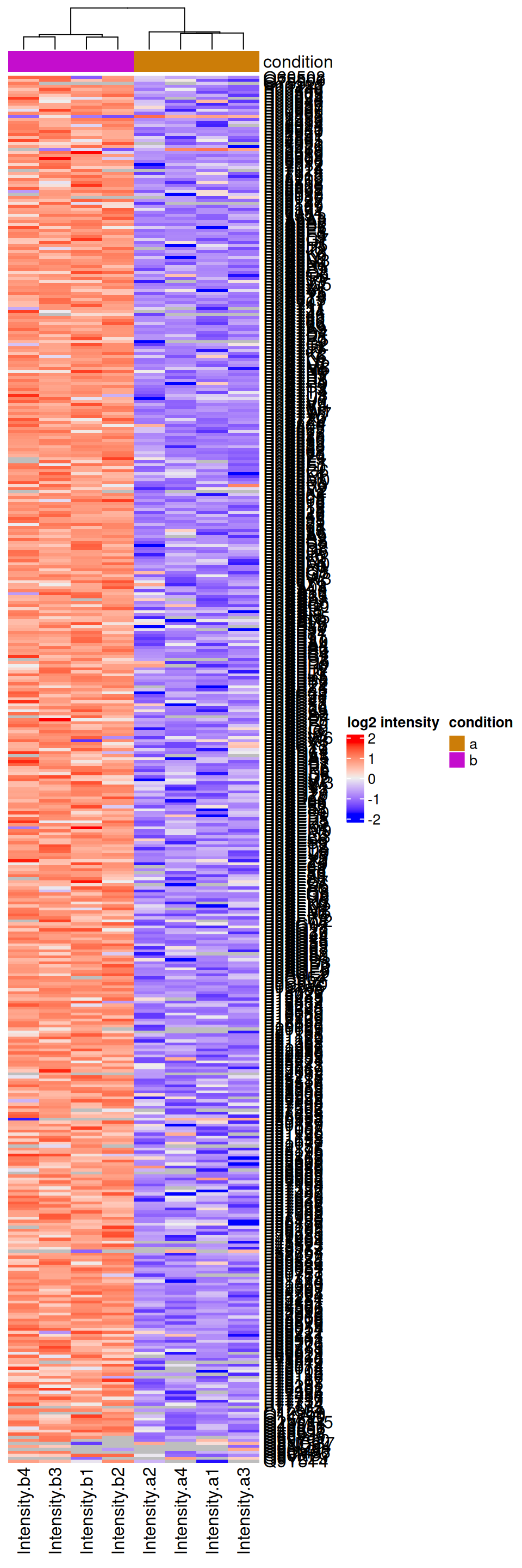
We observe that the majority of the returned proteins are indeed upregulated in the higher spike-in condition b.
1.7.4 Fold change distributions
As this is a spike-in study with known ground truth, we can also plot the log2 fold change distributions against its true values, in this case 0 for the human proteins and 0.585 for the E. coli proteins.
ggplot(inference) +
  aes(y = logFC,
      x = isEcoli,
      colour = isEcoli) +
  geom_boxplot() +
  geom_hline(yintercept = c(0, log2(4.5) - log2(3)),
             colour = c("grey20", "firebrick")) +
  scale_color_manual(
    values = c("grey20", "firebrick"), name = "",
    labels = c("Human proteins", "E. coli proteins")
  ) +
  ggtitle(paste0("Hypothesis test: ", colnames(L), " = 0"))
Warning: Removed 209 rows containing non-finite outside the scale range
(`stat_boxplot()`).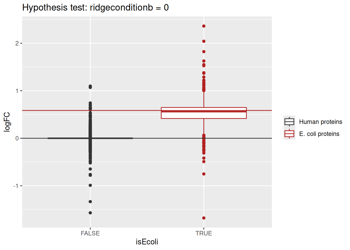
Estimated log2 fold change for human proteins are closely distributed around 0, as expected. log2 fold changes for E. coli proteins are distributed around the fold changes induced by the experimental design, indicating that msqrob2 is providing unbiased fold change estimates.
1.7.5 Detail plots
We can explore the data for a protein to validate the statistical inference results. For example, let’s explore the peptide and the summarised protein intensities for the protein with the most significant difference.
(targetProtein <- rownames(inference)[which.min(inference$adjPval)])[1] "P0A799"To obtain the required data, we perform a little data manipulation pipeline:
We use the QFeatures subsetting functionality to retrieve all data related to and focusing on the peptides_log and proteins sets that contains the peptide ion data used for model fitting. We then convert the data with longForm() for plotting. Finally, we plot the log2 normalised intensities for each sample at the protein and at the peptide level. Since multiple peptides are recorded for the protein, we link peptides across samples using a grey line. Samples are colored according to E. coli spike-in condition.
spikein[targetProtein, , c("peptides_log", "proteins")] |> #1
  longForm(colvars = colnames(colData(spikein)), #2
           rowvars = "Proteins") |>
  data.frame() |>
  ggplot() +
  aes(x = colname,
      y = value) +
  geom_line(aes(group = rowname), linewidth = 0.1) +
  geom_point(aes(colour = condition)) +
  facet_wrap(~ assay, scales = "free") +
  ggtitle(targetProtein) +
  theme_minimal() +
  theme(axis.text.x = element_blank())
Warning: 'experiments' dropped; see 'drops()'harmonizing input:
removing 40 sampleMap rows not in names(experiments)Warning: Removed 12 rows containing missing values or values outside the scale range
(`geom_line()`).Warning: Removed 34 rows containing missing values or values outside the scale range
(`geom_point()`).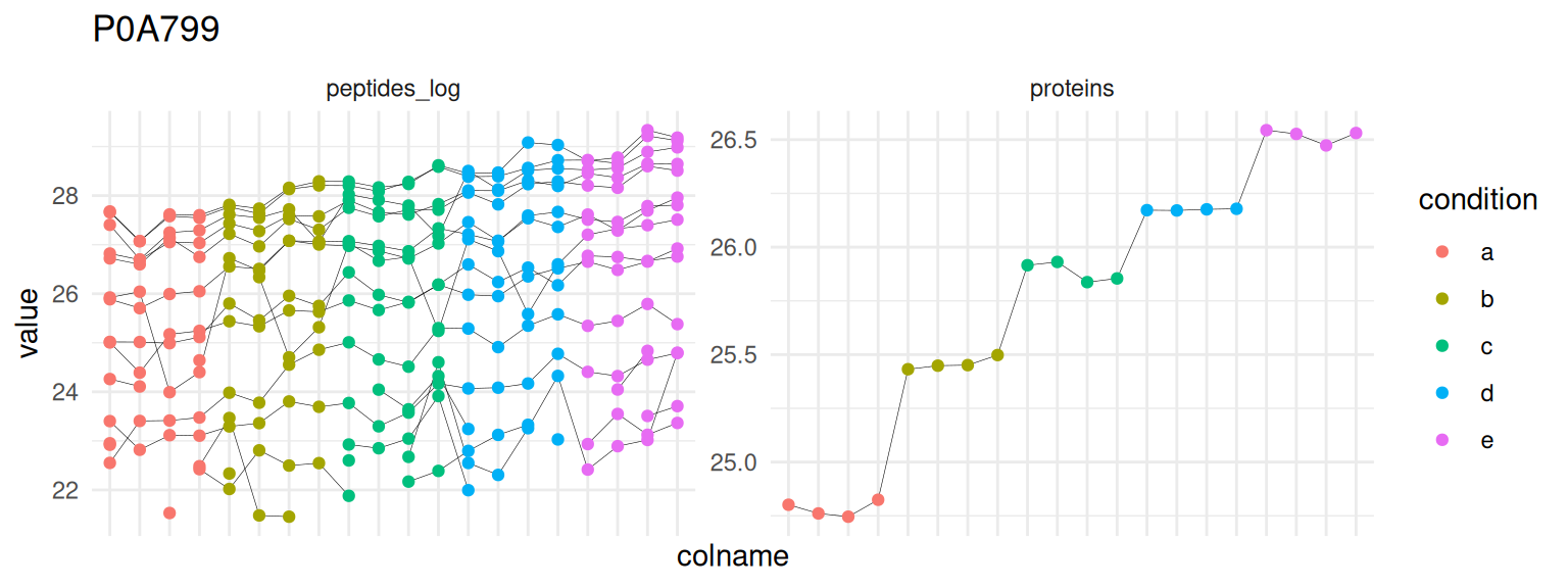
1.8 Going further
1.8.1 Testing muliple contrasts at once
We showed how to perform a hypothesis test to answer the question “which proteins change in abundance between condition b and condition a?”. However, since we have 5 conditions, we can do further comparisons. msqrob2 can assess multiple hypothesis at once. Like above we must provide which hypotheses we want to compare. createPairwiseContrasts() will generate all possible comparisons between condition level. The function requires the model specification that has been estimated and the sample annotation from the data. We also specify that we estimated the model using ridge regression, which influences parameter names.
(allHypotheses <- createPairwiseContrasts(
  model,
  colData(spikein),
  "condition"
))
Warning: the 'nobars' function has moved to the reformulas package. Please update your imports, or ask an upstream package maintainter to do so.
This warning is displayed once per session. [1] "conditionb = 0" "conditionc = 0"
[3] "conditiond = 0" "conditione = 0"
[5] "conditionc - conditionb = 0" "conditiond - conditionb = 0"
[7] "conditione - conditionb = 0" "conditiond - conditionc = 0"
[9] "conditione - conditionc = 0" "conditione - conditiond = 0"We now run the same workflow as above for a single hypothesis, except that here allHypotheses is a vector of contrasts.
(L <- makeContrast(
  allHypotheses,
  parameterNames = paste0("condition", c("b", "c", "d", "e"))
))
conditionb conditionc conditiond conditione conditionc - conditionb
conditionb 1 0 0 0 -1
conditionc 0 1 0 0 1
conditiond 0 0 1 0 0
conditione 0 0 0 1 0
conditiond - conditionb conditione - conditionb
conditionb -1 -1
conditionc 0 0
conditiond 1 0
conditione 0 1
conditiond - conditionc conditione - conditionc
conditionb 0 0
conditionc -1 -1
conditiond 1 0
conditione 0 1
conditione - conditiond
conditionb 0
conditionc 0
conditiond -1
conditione 1The contrast contains multiple hypotheses (multiple column) that involve multiple parameters (multiple rows).
We use again hypothesisTest() for performing the hypothesis test. We already generated results for the contrast ridgeconditionb = 0 and the function will throw an error by default, but we can overwrite the results with the argument overwrite = TRUE.
spikein <- hypothesisTest(spikein, i = "proteins", L, overwrite = TRUE)The results tables for the contrast are stored in the row data of the proteins assay in spikein under the colomnames of the contrast matrix L.
Users can directly access the results tables via de colData. However, msqrob2 also provides the msqrobCollect function. This function will automatically retrieve the results tables for all contrasts in contrast matrix L and combine them by default in one table. This table contains two additional columns: contrast with the name of the contrast and feature with the name of the modelled feature, here protein.
inferences <-
  msqrobCollect(spikein[["proteins"]], L)
head(inferences)
logFC se df t pval
conditionb.A0AVT1 0.10494859 0.07901174 15.963899 1.3282658 0.2027682
conditionb.A0FGR8 0.06906717 0.04535794 16.141441 1.5227140 0.1471798
conditionb.A0MZ66 -0.10892095 0.06295311 16.313394 -1.7301916 0.1024661
conditionb.A1L0T0 -0.02486814 0.18978721 16.791528 -0.1310317 0.8973073
conditionb.A1X283 -0.15880954 0.44509882 5.288059 -0.3567962 0.7350432
conditionb.A2RRP1 -0.12957365 0.09296872 14.972800 -1.3937339 0.1837409
adjPval contrast feature
conditionb.A0AVT1 0.6845834 conditionb A0AVT1
conditionb.A0FGR8 0.5908265 conditionb A0FGR8
conditionb.A0MZ66 0.4872344 conditionb A0MZ66
conditionb.A1L0T0 0.9858930 conditionb A1L0T0
conditionb.A1X283 0.9680034 conditionb A1X283
conditionb.A2RRP1 0.6617389 conditionb A2RRP1We rename the contrasts by removing the string ‘ridgecondition’.
inferences$contrast <- gsub("condition","", inferences$contrast)We add the ground truth as we know that E. coli is spiked in:
inferences$isEcoli <- inferences$feature %in% ecoliWe plot the volcano plots with each comparison in a separate facet and again color the dots according to the ground truth.
inferences |>
  plotVolcano() +
    aes(color = isEcoli, shape = adjPval < alpha) +
    scale_color_manual(
      values = c("grey20", "firebrick"),
      name = "species",
      labels = c("human", "ecoli")
      ) +
  labs(shape = paste0("FDR < ",alpha)) +
  facet_wrap(~ contrast)
Scale for colour is already present.
Adding another scale for colour, which will replace the existing scale.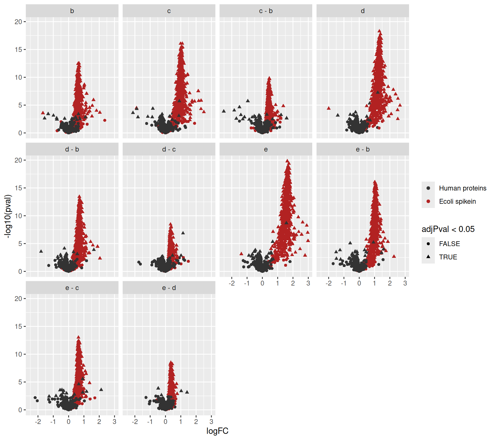
Since we know the ground truth we can again evaluate the number of true positives, false positives and false discovery proportion.
inferences |>
  filter(adjPval < 0.05) |>
  group_by(contrast) |>
  summarise(
    fp = sum(!isEcoli),
    tp = sum(isEcoli),
    fdp = round(mean(!isEcoli)*100,2))
# A tibble: 10 × 4
contrast fp tp fdp
<chr> <int> <int> <dbl>
1 b 21 447 4.49
2 c 42 543 7.18
3 c - b 27 320 7.78
4 d 57 587 8.85
5 d - b 46 514 8.21
6 d - c 8 234 3.31
7 e 97 611 13.7
8 e - b 82 581 12.4
9 e - c 40 506 7.33
10 e - d 7 265 2.57If the FDR is well controlled, we expect the FDPs to fluctuate around the nominal FDR level of 5%. We observe, however,that the FDPs for the contrasts envolving larger fold changes e.g e (e vs a) and (e vs b) are much larger than 5%, indicating that the results might be too liberal for these comparisons. Note, that this is often seen in spike-in studies where all proteins that are spiked in are regulated in the same direction, which can lead to ion suppression for the non-DA proteins in high spike-in samples and puts a burden on the normalisation assumptions. We will illustrate in later chapters Benchmarking workflows and Optimisation of a data analysis workflow that more robust inference for this dataset can be provided with ridge regression. However, this comes at a considerable computational cost.
We can also assess the fold changes, but we first create a small table with the real values.
realLogFC <- data.frame(
  logFC = t(L) %*% lm(log2(concentration) ~ condition, colData(spikein))$coef[-1]
)
realLogFC$contrast <- gsub("condition","",colnames(L))
We can now create the boxplots with the estimated log2-fold changes, adding horizontal lines with the corresponding target values.
inferences |>
  na.exclude() |>
  ggplot(
    aes(y = logFC,
        x = isEcoli,
        colour = isEcoli)) +
  geom_boxplot()  +
  scale_color_manual(
    values = c("grey20", "firebrick"), name = "",
    labels = c("Human proteins", "E. coli proteins")
  ) +
  facet_wrap(~contrast) +
  geom_hline(data = realLogFC, aes(yintercept = logFC),
             colour = "firebrick") +
  geom_hline(yintercept = 0)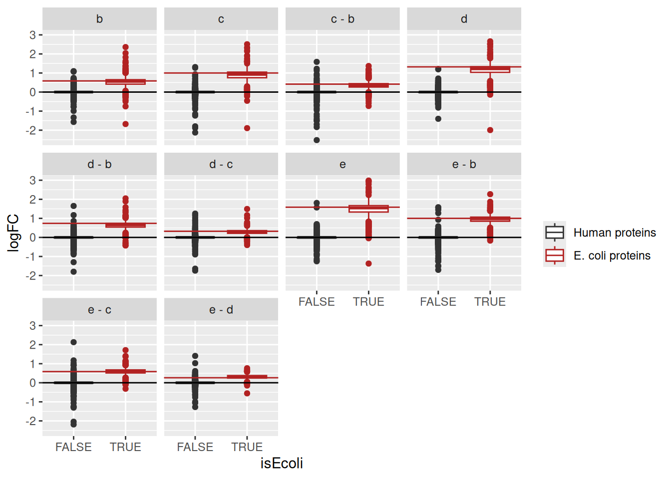
We again observe that the log2 fold change estimates are close to the real spike-in fold changes induced by the experimental design.
1.8.2 Model the spike-in concentration as a numeric
Since the relative concentration of the E. coli spike-in lysate is known, we can also model the effect of the treatment using the log2-transformed spike-in concentration as a continuous covariate. We then expect the slope to be close to 1 for E. coli proteins.
- We first create a variable with log2 transformed concentration in the
colData. - We fit an msqrob model using the log2 transformed concentration as a fixed effect. Note, that we set
ridge = FALSEbecause we only have one slope parameter in the model. We store the models in a new column with name"concentration_model". - We setup a contrast for the slope term.
- We conduct the hypothesis test for all proteins.
spikein$concentration_log2 <- log2(spikein$concentration) #1.
spikein <- msqrob( #2.
  spikein, i = "proteins",
  formula = ~ concentration_log2,
  ridge = FALSE,
  robust = TRUE,
  modelColumnName = "concentration_model"
)
L <- makeContrast( #3.
  "concentration_log2 = 0", parameterNames = "concentration_log2"
)
spikein <- hypothesisTest( #4.
  spikein, i = "proteins", L, modelColumn = "concentration_model",
  overwrite = TRUE
)
We plot the results using the volcano plot as in the previous section.
inferenceLin <- msqrobCollect(spikein[["proteins"]], L)
inferenceLin$isEcoli <- inferenceLin$feature %in% ecoli
plotVolcano(inferenceLin) +
  aes(color = isEcoli, shape = adjPval < alpha) +
  scale_color_manual(
    values = c("grey20", "firebrick"),
    name = "species",
    labels = c("human", "ecoli")
    ) +
  geom_vline(xintercept = 1, linetype = "dashed")
Scale for colour is already present.
Adding another scale for colour, which will replace the existing scale.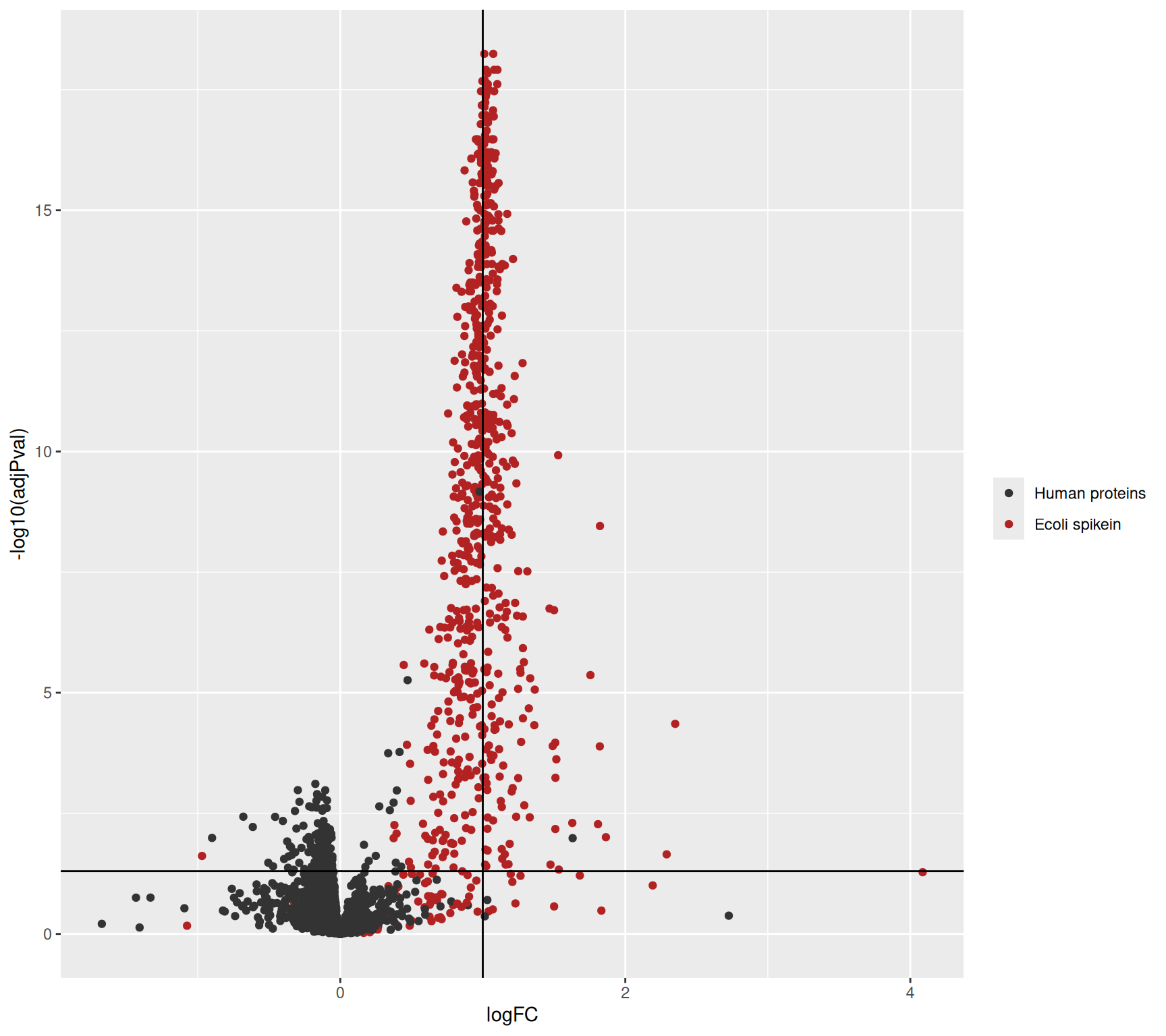
logFC actually stands for the slope parameter.Similarly, we plot the estimated log2 concentration slope against the expected value.
inferenceLin |>
  na.exclude() |>
  ggplot(
    aes(y = logFC,
        x = isEcoli,
        colour = isEcoli)) +
  geom_boxplot()  +
  scale_color_manual(
    values = c("grey20", "firebrick"), name = "",
    labels = c("Human proteins", "E. coli proteins")
  ) +
  geom_hline(yintercept = 0) +
  geom_hline(yintercept = 1, color = "firebrick")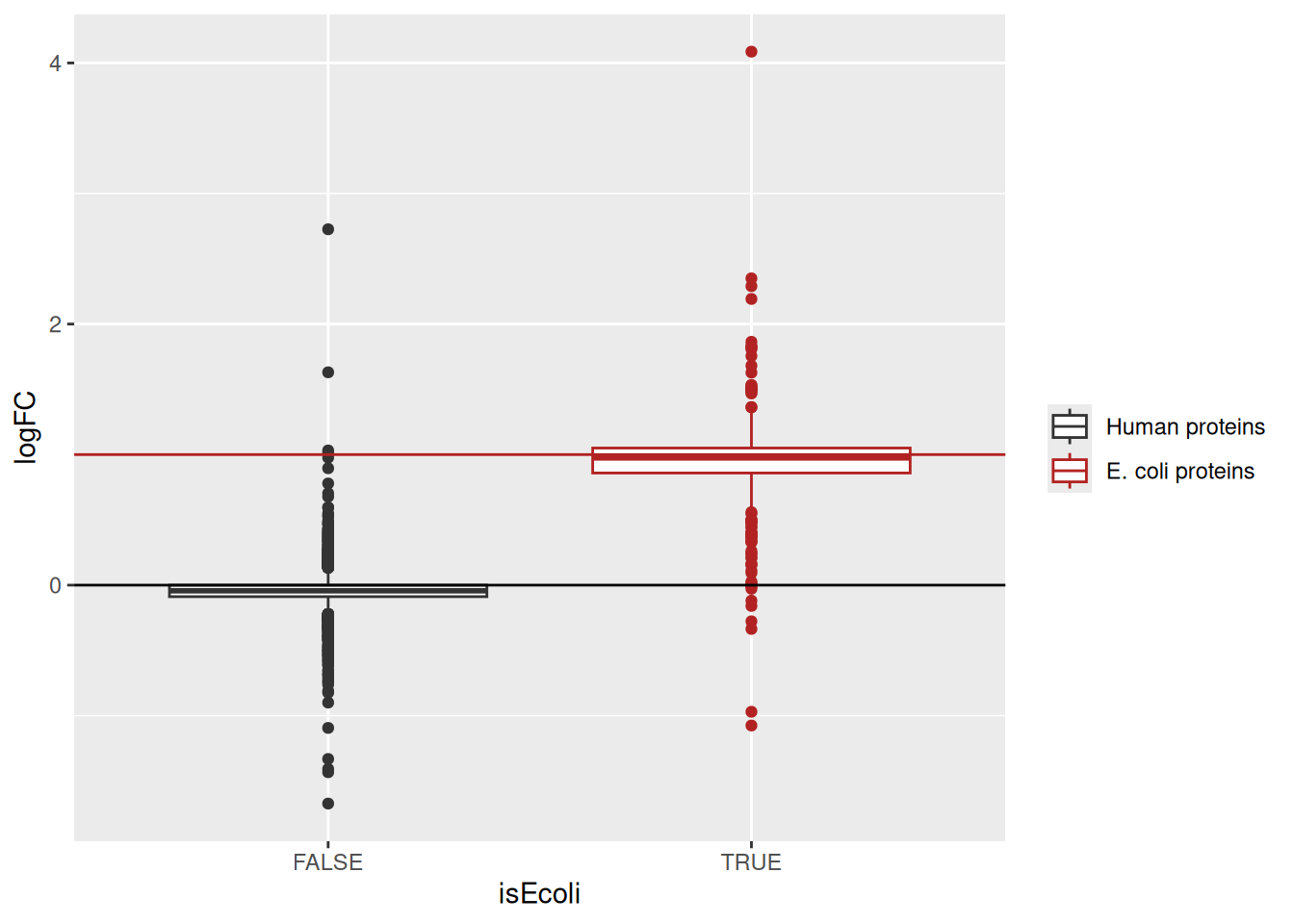
Note, that the slopes for the human and E. coli proteins are centered around 0 and 1, respectively.
1.9 Conclusion
In this vignette, we have demonstrated a typical data analysis workflow for label free data using msqrob2. Because the packages relies on the QFeatures data class, we could demonstrate the implementation of a complete pre-processing workflow starting from MaxQuant’s peptide table: log2-transformation, PSM filtering, missing value management, normalisation, and summarisation. The data exploration revealed expected patterns of variation among samples, as this is a ground truth data set.
Once pre-processed, we use the msqrob2 package to model the (known) effect of spike-in condition. We showed how to run statistical inference on the modelling results to retrieve the significance of differentially abundant proteins. We explored statistical results through volcano plots and boxplots of the log2 fold changes and visually validated the results for one protein by plotting the input data. We have shown the inference pipeline can be streamlined when assessing multiple hypotheses. In this example, the spike-in condition can be encoded as a categorical variable or a numeric variable, and we showed how to model and interpret the results for both cases.
This chapter thus provides a general framework for analysing simple experimental designs for label-free proteomics experiments. Remember, this book provides an overview of different use-cases with more complex designs. In the next chapter, we will illustrate advanced concepts of proteomics data analysis, illustrated by the analysis of a TMT-labelled spike-in experiment.
The ion selection for MS2 depends on the data recorded in MS1. Therefore, this approach is referred to as data dependent acquisition (DDA).↩︎
MaxQuant also computes a protein table. However, we found that starting from MaxQuant’s protein table leads to a decrease in performance. We will illustrate in this tutorial how to build the protein table.↩︎
Improving peptide identification is outside the scope of this tutorial↩︎
Recall that only the top most intense ion peaks are send for MS2↩︎
A
QFeaturesobject can be seen as a special list ofSummarizedExperimentobjects.↩︎see also the R for mass spectrometry book↩︎
We will however not evaluate the code in this tutorial as our general advice is to avoid imputation. To run the code, you’ll need to uncomment it first.↩︎
We will explain this with more details at the end of the summarisation step↩︎
During robust estimation, the least squared error minimisation, that is minimising \(\sum_i\mathbf{\epsilon}^2_i\), is iteratively reweighted using Huber weights, i.e. \(\sum_iw_i\mathbf{\epsilon}^2_i\). This is internally performed using
MASS::rlm().↩︎In fact, this is also true for the previous transformation where the peptides are linked across sets.↩︎
Recall that a to e condition imply low to high concentration.↩︎
Note that we have the spike-in concentration encoded in two ways.
concentrationis encoded as a numerical value and provides the actual concentration amount in fmol/µL.conditionis encoded as a factor, meaning that every concentration is regarded as an independent group. We will use the latter encoding as most common research questions consist of group-wise comparisons. The modelling of concentration as a numeric will be discussed in a dedicated section↩︎Categorical variables are encoded using dummy coding.↩︎
We don’t need to specify the intercept as R automatically adds it during model estimation. you can explicitly add it using
~ 1 + ..., you can also suppress it using~ 0 +. When an intercept is included, one of the groups is defined as the reference group and its corresponding model parameter is absorbed in the intercept. The residuals don’t need to be specified as they are part of the model estimation process.↩︎Note, that we only need to specify the names of the model parameters that are involved in the contrast when using the make contrast function. The hypothesisTest function below will then subset the relevant part from the model output. Also, note that the contrast matrix in this example is trivial. However, we will later show how to asses multiple hypotheses at once and then the contrast matrix consists of multiple columns, with one column for each contrast↩︎
Note, that upon this transformation a value of 1 represents a p-value of 0.1, 2 a p-value of 0.01, 3 a p-value of 0.001, etc.↩︎
The
scales()function aligns the means and the centered standard deviations by column. Since we want to scale by row, we need to transpose (t())) before scaling and transpose back after scaling. Scaling the data will remove changes in feature intensities that are caused by uninteresting changes in ionisation efficiency.↩︎