Recap general linear model

This is part of the online course Statistical Genomics 2022 (SGA)

1 Breast cancer example

• part of study https://doi.org/10.1093/jnci/djj052)
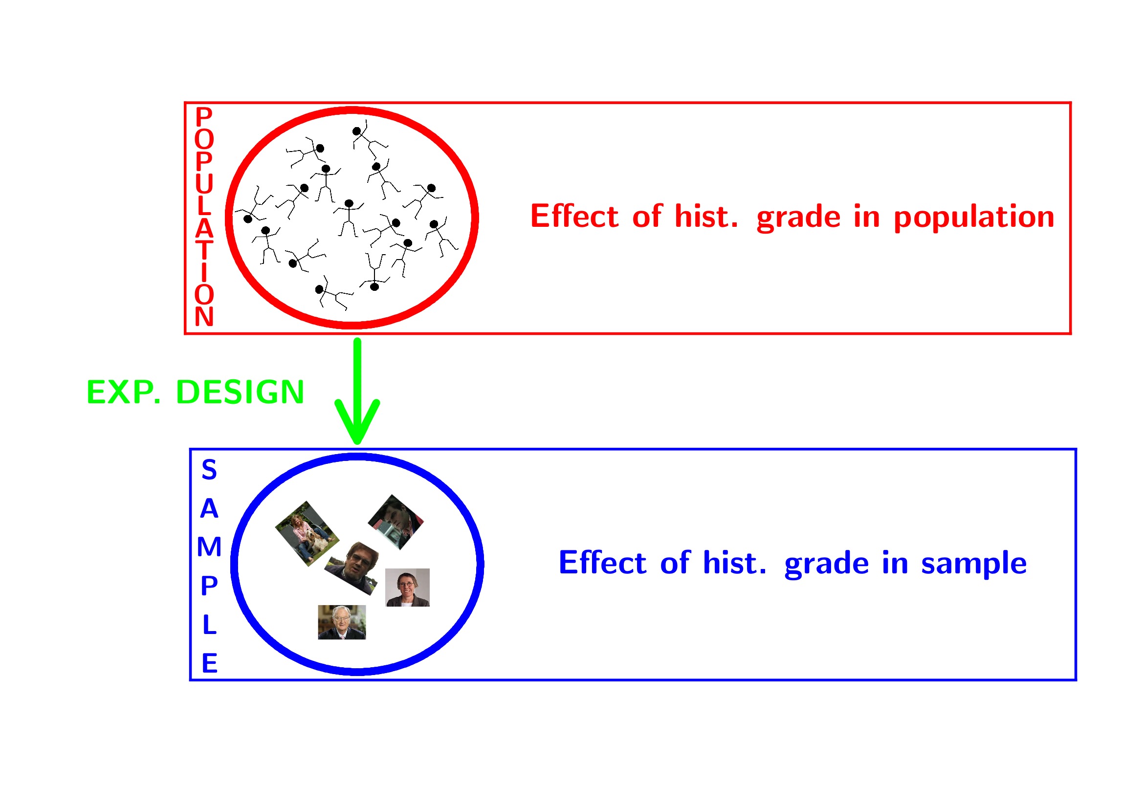
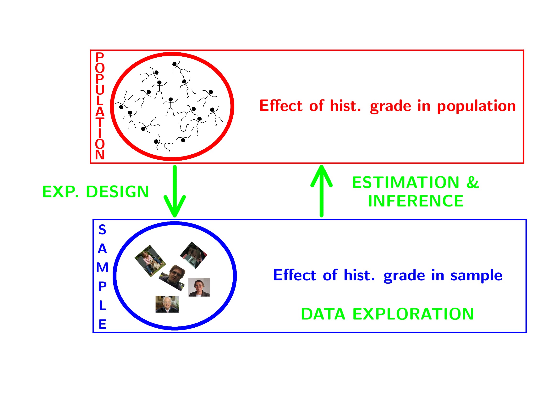
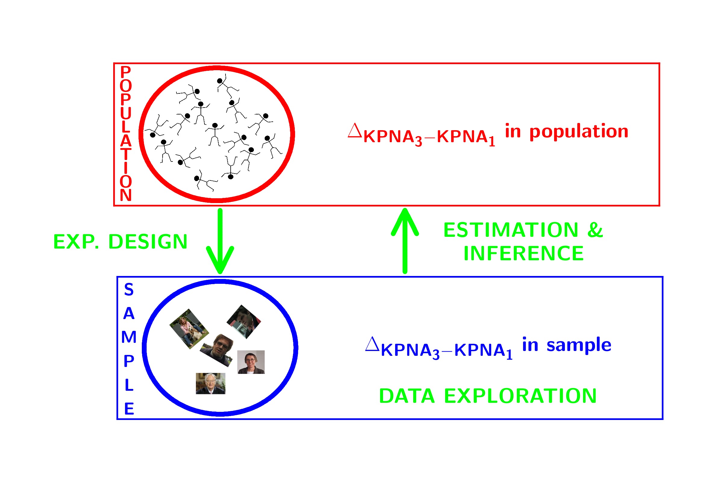
• Histologic grade in breast cancer clinically prognostic. Association of histologic grade on expression of KPNA2 gene that is known to be associated with poor BC prognosis.
• Population: all current and future breast cancer patients

---

---

---

---

---

---

2 Data Exploration

2.1 Import

library(tidyverse)

## ── Attaching core tidyverse packages ──────────────────────── tidyverse 2.0.0 ──
## ✔ dplyr     1.1.4     ✔ readr     2.1.5
## ✔ forcats   1.0.0     ✔ stringr   1.5.1
## ✔ ggplot2   3.5.1     ✔ tibble    3.2.1
## ✔ lubridate 1.9.3     ✔ tidyr     1.3.1
## ✔ purrr     1.0.2     
## ── Conflicts ────────────────────────────────────────── tidyverse_conflicts() ──
## ✖ dplyr::filter() masks stats::filter()
## ✖ dplyr::lag()    masks stats::lag()
## ℹ Use the conflicted package (<http://conflicted.r-lib.org/>) to force all conflicts to become errors

gene <- read.table("https://raw.githubusercontent.com/statOmics/SGA21/master/data/kpna2.txt",header=TRUE)
head(gene)

We will transform the variable grade and node to a factor

gene$grade <- as.factor(gene$grade)
gene$node <- as.factor(gene$node)

2.2 Summary statistics

geneSum <- gene %>%
  group_by(grade) %>%
  summarize(mean = mean(gene),
            sd = sd(gene),
            n=length(gene)
            ) %>%
  mutate(se = sd/sqrt(n))
geneSum

2.3 Visualisation

gene %>%
  ggplot(aes(x=grade,y=gene)) +
  geom_boxplot(outlier.shape=NA) +
  geom_jitter()

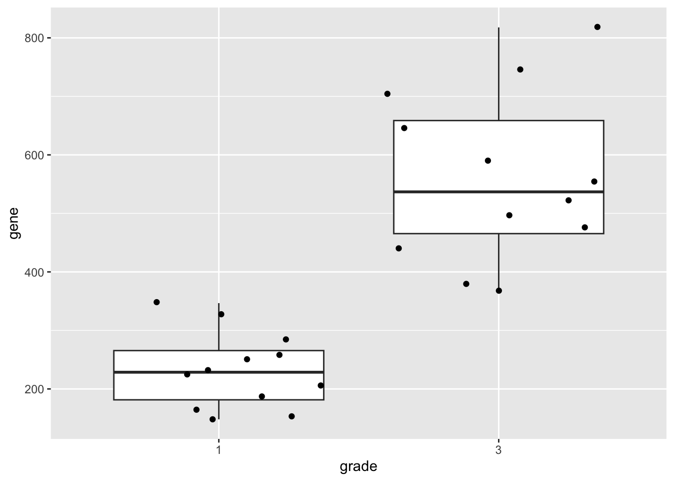
We can also save the plots as objects for later use!

p1 <- gene %>%
  ggplot(aes(x=grade,y=gene)) +
  geom_boxplot(outlier.shape=NA) +
  geom_jitter()

p2 <- gene %>%
  ggplot(aes(sample=gene)) +
  geom_qq() +
  geom_qq_line() +
  facet_wrap(~grade)

p1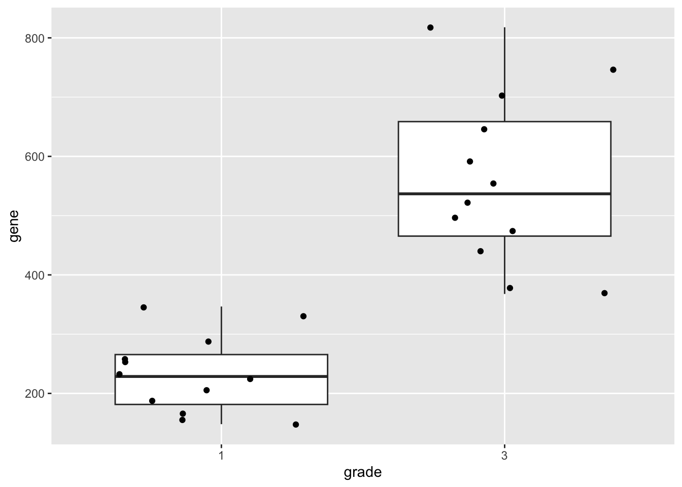

p2

2.4 Research questions

Researchers want to assess the association of the histological grade on KPNA2 gene expression

---

2.5 Estimation of effect size and standard error

effectSize <- tibble(
  delta = geneSum$mean[2]- geneSum$mean[1],
  seDelta = geneSum %>%
    pull(se) %>%
    .^2 %>%
    sum %>%
    sqrt
  )
effectSize

3 Statistical Inference

• Researchers want to assess the association of histological grade on KPNA2 gene expression
• Inference?

---

---

• Researchers want to assess the association of histological grade on KPNA2 gene expression
• Inference?
• testing + CI $ $ Assumptions

---

• In general we start from alternative hypothese \(H_A\): we want to show an association

• Gene expression of grade 1 and grade 3 patients is on average different

• But, we will assess it by falsifying the opposite:

• The average KPNA2 gene expression of grade 1 and grade 3 patients is equal

---

• How likely is it to observe an equal or more extreme association than the one observed in the sample when the null hypothesis is true?

• When we make assumptions about the distribution of our test statistic we can quantify this probability: p-value.

• If the p-value is below a significance threshold \(\alpha\) we reject the null hypothesis

We control the probability on a false positive result at the \(\alpha\)-level (type I error)

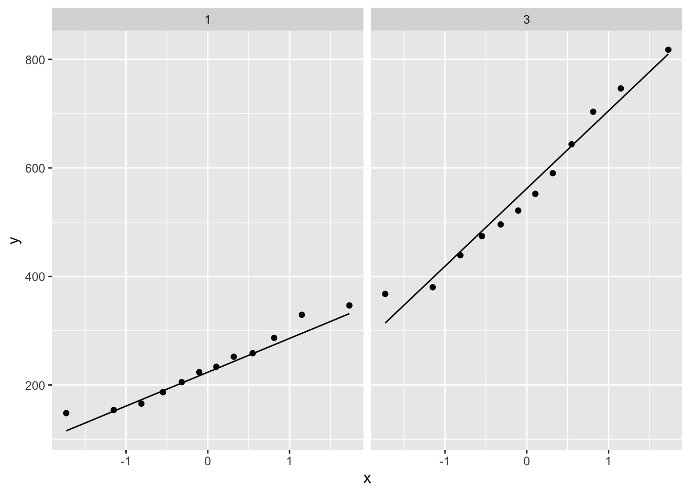
• The p-value will only be calculated correctly if the underlying assumptions hold!

library(gridExtra)

## 
## Attaching package: 'gridExtra'

## The following object is masked from 'package:dplyr':
## 
##     combine

p1

p2

t.test(gene~grade,data=gene)

## 
##  Welch Two Sample t-test
## 
## data:  gene by grade
## t = -7.2132, df = 15.384, p-value = 2.598e-06
## alternative hypothesis: true difference in means between group 1 and group 3 is not equal to 0
## 95 percent confidence interval:
##  -425.4218 -231.6751
## sample estimates:
## mean in group 1 mean in group 3 
##        232.5003        561.0487

effectSize <- effectSize %>%
  mutate(t.stat=delta/seDelta) %>%
  mutate(p.value= pt(-abs(t.stat),21.352)*2)

effectSize

• Intensities are often not normally distributed and have a mean variance relation
• Commonly log2-transformed
• Differences on log scale:

\[ \log_2(B) - \log_2(A) = \log_2 \frac{B}{A} = \log_2 FC_{\frac{B}{A}} \]

---

3.1 Log transformation

gene <- gene %>%
  mutate(lgene = log2(gene))

p1 <- gene %>%
  ggplot(aes(x=grade,y=lgene)) +
  geom_boxplot(outlier.shape=NA) +
  geom_jitter()

p2 <- gene %>%
  ggplot(aes(sample=lgene)) +
  geom_qq() +
  geom_qq_line() +
  facet_wrap(~grade)

p1

p2

logtest <- t.test(lgene~grade,data=gene,var.equal=TRUE)
logtest

## 
##  Two Sample t-test
## 
## data:  lgene by grade
## t = -8.0455, df = 22, p-value = 5.372e-08
## alternative hypothesis: true difference in means between group 1 and group 3 is not equal to 0
## 95 percent confidence interval:
##  -1.610148 -0.950178
## sample estimates:
## mean in group 1 mean in group 3 
##        7.808478        9.088641

log2FC <- logtest$estimate[2]-logtest$estimate[1]
log2FC

## mean in group 3 
##        1.280163

names(log2FC) <- "g3-g1"
2^log2FC

##    g3-g1 
## 2.428664

3.2 Conclusion

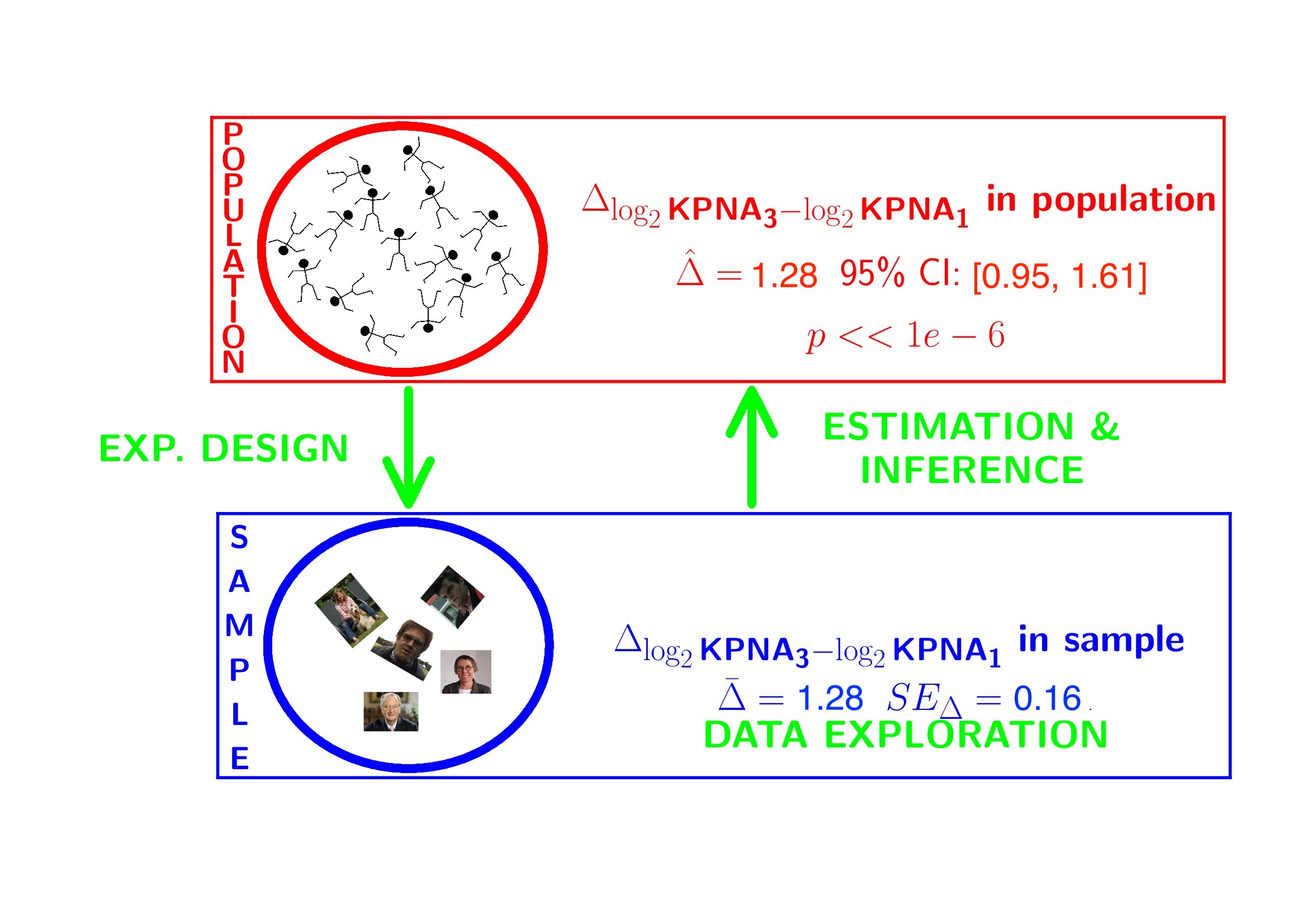
There is a extremely significant association of the histological grade on the gene expression in tumor tissue. On average, the gene expression for the grade 3 patients is 2.43 times higher than the gene expression in grade 1 patients (95% CI [1.93, 3.05], \(p<<0.001\)).

---

---

The patients also differ in the their lymph node status. Hence, we have a two factorial design: grade x lymph node status!!!

Solution??

---

4 General Linear Model

How can we integrate multiple factors and continuous covariates in linear model.

\[ y_i= \beta_0 + \beta_1 x_{i,1} + \beta_2 x_{i,2} + \beta_{12}x_{i,1}x_{i,2}+\epsilon_i, \] with

• \(x_{i,1}\) a dummy variable for histological grade: \(x_{i,1}=\begin{cases} 0& \text{grade 1}\\ 1& \text{grade 3} \end{cases}\)
• \(x_{i,2}\) a dummy variable for : \(x_{i,2}=\begin{cases} 0& \text{lymph nodes were not removed}\\ 1& \text{lymph nodes were removed} \end{cases}\)
• \(\epsilon_i\)?

---

4.1 Implementation in R

lm1 <- lm(gene~grade*node,data=gene)
summary(lm1)

## 
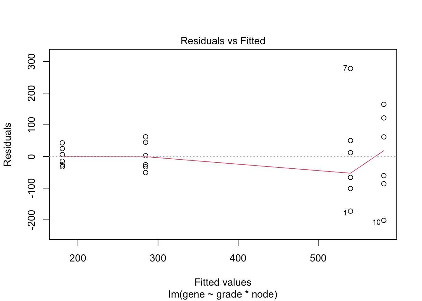
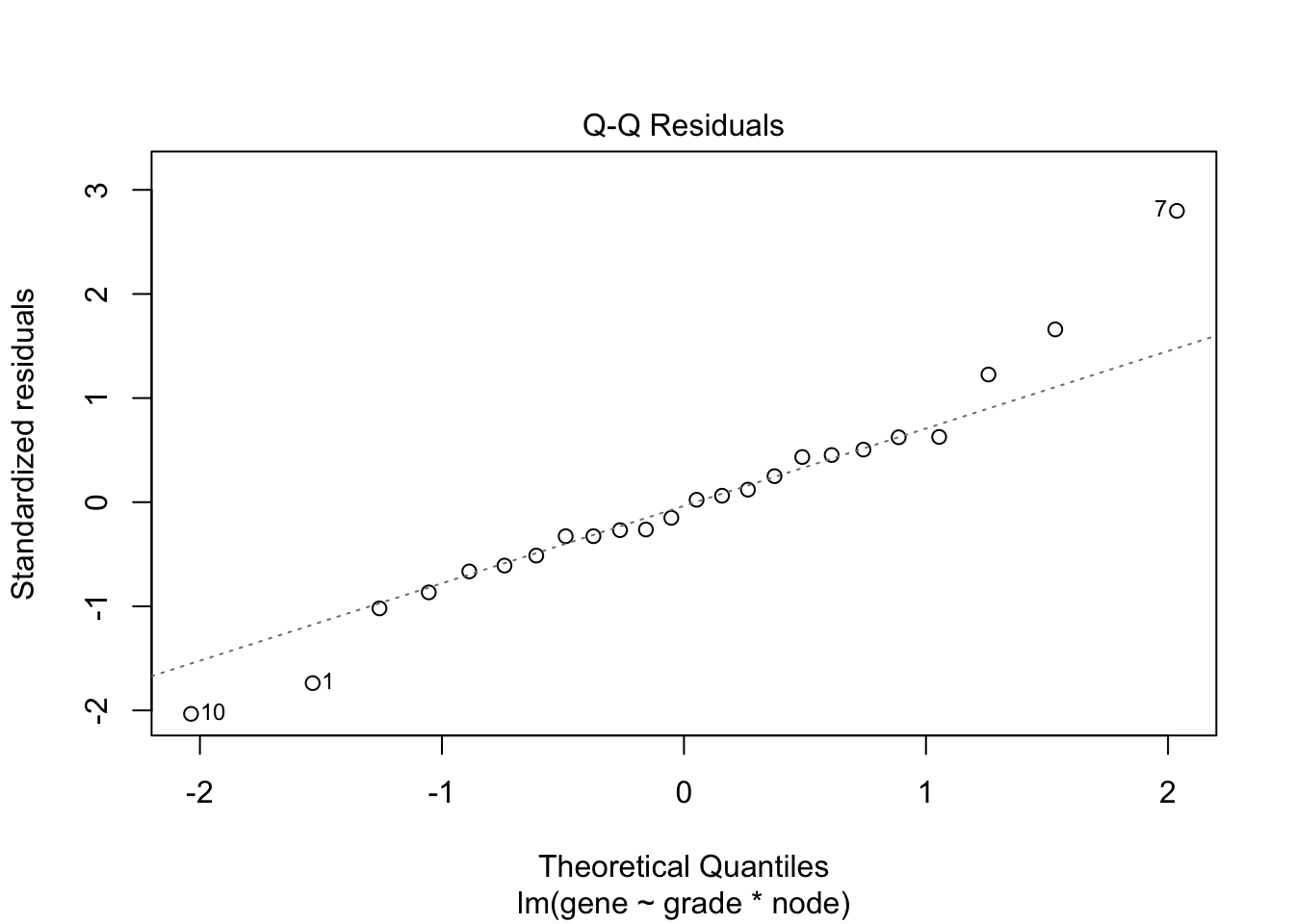
## Call:
## lm(formula = gene ~ grade * node, data = gene)
## 
## Residuals:
##      Min       1Q   Median       3Q      Max 
## -201.748  -53.294   -6.308   46.216  277.601 
## 
## Coefficients:
##              Estimate Std. Error t value Pr(>|t|)    
## (Intercept)    180.51      44.37   4.068   0.0006 ***
## grade3         401.33      62.75   6.396 3.07e-06 ***
## node1          103.98      62.75   1.657   0.1131    
## grade3:node1  -145.57      88.74  -1.640   0.1166    
## ---
## Signif. codes:  0 '***' 0.001 '**' 0.01 '*' 0.05 '.' 0.1 ' ' 1
## 
## Residual standard error: 108.7 on 20 degrees of freedom
## Multiple R-squared:  0.7437, Adjusted R-squared:  0.7052 
## F-statistic: 19.34 on 3 and 20 DF,  p-value: 3.971e-06

---

4.2 Assumptions

plot(lm1)

---

4.3 Breast cancer example

• Paper: https://doi.org/10.1093/jnci/djj052
• Histologic grade in breast cancer provides clinically important prognostic information. Two factors have to be concidered: Histologic grade (grade 1 and grade 3) and lymph node status (0 vs 1). The researchers assessed gene expression of the KPNA2 gene a protein-coding gene associated with breast cancer and are mainly interested in the association of histological grade. Note, that the gene variable consists of background corrected normalized intensities obtained with a microarray platform. Upon log-transformation, they are known to be a good proxy for the \(\log\) transformed concentration of gene expression product of the KPNA2 gene.
• Research questions and translate them towards model parameters (contrasts)?
• Make an R markdown file to answer the research questions

library(ExploreModelMatrix)
explMx <- VisualizeDesign(gene,designFormula = ~grade*node)
explMx$plotlist

## [[1]]

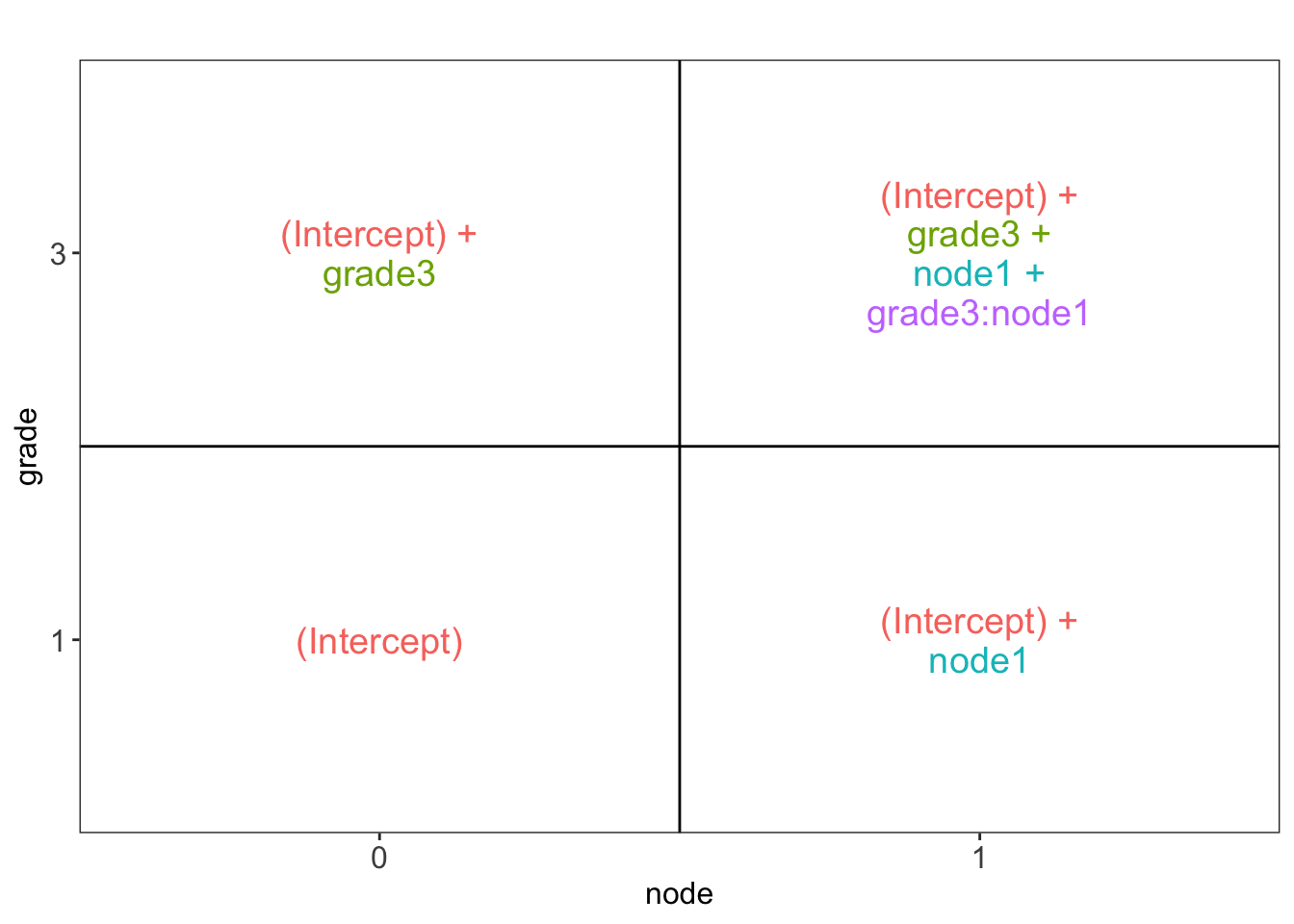
You can also explore the model matrix interactively:

ExploreModelMatrix(gene,designFormula = ~grade*node)

---

5 Linear regression in matrix form

5.1 Scalar form

• Consider a vector of predictors \(\mathbf{x}=(x_1,\ldots,x_p)^T\) and
• a real-valued response \(Y\)
• then the linear regression model can be written as \[ Y=f(\mathbf{x}) +\epsilon=\beta_0+\sum\limits_{j=1}^p x_j\beta_j + \epsilon \] with i.i.d. \(\epsilon\sim N(0,\sigma^2)\)

5.2 Matrix form

• \(n\) observations \((\mathbf{x}_1,y_1) \ldots (\mathbf{x}_n,y_n)\)
• Regression in matrix notation \[\mathbf{Y}=\mathbf{X\beta} + \mathbf{\epsilon}\] with \(\mathbf{Y}=\left[\begin{array}{c}y_1\\ \vdots\\y_n\end{array}\right]\), \(\mathbf{X}=\left[\begin{array}{cccc} 1&x_{11}&\ldots&x_{1p}\\ \vdots&\vdots&&\vdots\\ 1&x_{n1}&\ldots&x_{np} \end{array}\right]\), \(\mathbf{\beta}=\left[\begin{array}{c}\beta_0\\ \vdots\\ \beta_p\end{array}\right]\) and \(\mathbf{\epsilon}=\left[\begin{array}{c} \epsilon_1 \\ \vdots \\ \epsilon_n\end{array}\right]\)

5.3 Least Squares (LS)

• Minimize the residual sum of squares \[\begin{eqnarray*} RSS(\mathbf{\beta})&=&\sum\limits_{i=1}^n e^2_i\\ &=&\sum\limits_{i=1}^n \left(y_i-\beta_0-\sum\limits_{j=1}^p x_{ij}\beta_j\right)^2 \end{eqnarray*}\]
• or in matrix notation \[\begin{eqnarray*} RSS(\mathbf{\beta})&=&(\mathbf{Y}-\mathbf{X\beta})^T(\mathbf{Y}-\mathbf{X\beta})\\ &=&\Vert \mathbf{Y}-\mathbf{X\beta}\Vert^2_2 \end{eqnarray*}\] with the \(L_2\)-norm of a \(p\)-dim. vector \(v\) \(\Vert \mathbf{v} \Vert=\sqrt{v_1^2+\ldots+v_p^2}\) \(\rightarrow\) \(\hat{\mathbf{\beta}}=\text{argmin}_\beta \Vert \mathbf{Y}-\mathbf{X\beta}\Vert^2_2\)

---

5.3.1 Minimize RSS

\[ \begin{array}{ccc} \frac{\partial RSS}{\partial \mathbf{\beta}}&=&\mathbf{0}\\\\ \frac{(\mathbf{Y}-\mathbf{X\beta})^T(\mathbf{Y}-\mathbf{X\beta})}{\partial \mathbf{\beta}}&=&\mathbf{0}\\\\ -2\mathbf{X}^T(\mathbf{Y}-\mathbf{X\beta})&=&\mathbf{0}\\\\ \mathbf{X}^T\mathbf{X\beta}&=&\mathbf{X}^T\mathbf{Y}\\\\ \hat{\mathbf{\beta}}&=&(\mathbf{X}^T\mathbf{X})^{-1}\mathbf{X}^T\mathbf{Y} \end{array} \]

---

5.3.2 Geometric Interpretation

5.3.2.1 Toy dataset

We will illustrate this on a toy dataset

library(tidyverse)
data <- data.frame(x=1:3,y=c(1,2,2))
data

5.3.2.2 Matrix form for toy dataset

We can also write this in matrix form

\[ \mathbf{Y} = \mathbf{X}\boldsymbol{\beta}+\boldsymbol{\epsilon} \]

with

\[ \mathbf{Y}=\left[ \begin{array}{c} 1\\ 2\\ 2\\ \end{array}\right], \quad \mathbf{X}= \left[ \begin{array}{cc} 1&1\\ 1&2\\ 1&3\\ \end{array} \right], \quad \boldsymbol{\beta} = \left[ \begin{array}{c} \beta_0\\ \beta_1\\ \end{array} \right] \quad \text{and} \quad \boldsymbol{\epsilon}= \left[ \begin{array}{c} \epsilon_1\\ \epsilon_2\\ \epsilon_3 \end{array} \right] \]

5.3.2.3 Classical interpretation

Model fit and predictions based on the toy dataset

lm1 <- lm(y~x,data)
data$yhat <- lm1$fitted

data %>%
  ggplot(aes(x,y)) +
  geom_point() +
  ylim(0,4) +
  xlim(0,4) +
  stat_smooth(method = "lm", color = "red", fullrange = TRUE) +
  geom_point(aes(x=x, y =yhat), pch = 2, size = 3, color = "red") +
  geom_segment(data = data, aes(x = x, xend = x, y = y, yend = yhat), lty = 2 )

## `geom_smooth()` using formula = 'y ~ x'

## Warning in max(ids, na.rm = TRUE): no non-missing arguments to max; returning
## -Inf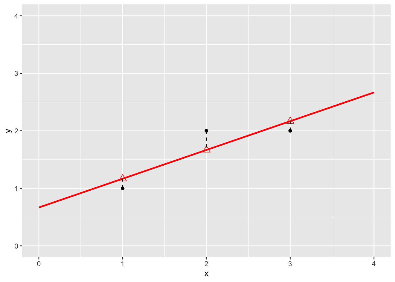

5.3.3 Projection

There is also another picture to regression:

• Instead of plotting each observation \(i= 1 \ldots n\) as a data-point in \(\mathbb{R}^p\) with dimensions \(1 \ldots p\) for every variable/feature that is recorded for each observation

• We can also plot \(\mathbf{Y}\), \(\hat{\mathbf{Y}}\) and each column of \(\mathbf{X}\): \(\mathbf{X}_j\) with \(j=1 \ldots p\) as a vector in \(\mathbb{R}^n\) with dimensions \(1 \ldots n\) for every observation.

• In this representation linear regression can be interpreted as a projection of the vector \(\mathbf{Y}\) onto the subspace of \(\mathbb{R}^n\) that is spanned by the vectors for the predictors \(\mathbf{X}_1 \ldots \mathbf{X}_p\).

• The space \(\mathbf{X}_1 \ldots \mathbf{X}_p\) is also referred to as the column space of \(\mathbf{X}\), the space that consists of all linear combinations of the vectors of the predictors or columns \(\mathbf{X}_1 \ldots \mathbf{X}_p\).

5.3.3.1 Intermezzo: Projection of vector on X and Y axis

\[ \mathbf{e}=\left[\begin{array}{c} e_1\\e_2\end{array}\right], \mathbf{u}_1 = \left[\begin{array}{c} 1\\0\end{array}\right], \mathbf{u}_2 = \left[\begin{array}{c} 0\\1\end{array}\right] \]

## Warning: Using `size` aesthetic for lines was deprecated in ggplot2 3.4.0.
## ℹ Please use `linewidth` instead.
## This warning is displayed once every 8 hours.
## Call `lifecycle::last_lifecycle_warnings()` to see where this warning was
## generated.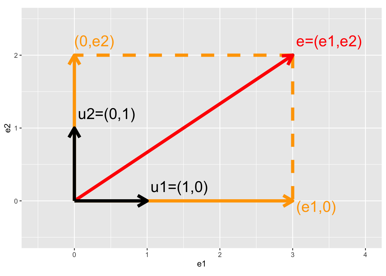

1. Projection of error on x-axis

\[\begin{eqnarray*} \mathbf{u}_1^T \mathbf{e} &=& \Vert \mathbf{u}_1\Vert_2 \Vert \mathbf{e}_1\Vert_2 \cos <\mathbf{u}_1,\mathbf{e}_1>\\ &=&\left[\begin{array}{cc} 1&0\end{array}\right] \left[\begin{array}{c} e_1\\e_2\end{array}\right]\\ &=& 1\times e_1 + 0 \times e_2 \\ &=& e_1\\ \end{eqnarray*}\]

2. Projection of error on y-axis

\[\begin{eqnarray*} \mathbf{u}_2^T \mathbf{e} &=& \left[\begin{array}{cc} 0&1\end{array}\right] \left[\begin{array}{c} e_1\\e_2\end{array}\right]\\ &=& 0\times e_1 + 1 \times e_2 \\ &=& e_2 \end{eqnarray*}\]

3. Projection of error on itself

\[\begin{eqnarray*} \mathbf{e}^T \mathbf{e} &=&\left[\begin{array}{cc} e_1&e_2\end{array}\right] \left[\begin{array}{c} e_1\\e_2\end{array}\right]\\ &=&e_1^2+e_2^2\\ &=&\Vert e \Vert^2_2 \rightarrow \text{ Pythagorean theorem} \end{eqnarray*}\]

---

5.3.3.2 Interpretation of least squares as a projection

Fitted values:

\[ \begin{array}{lcl} \hat{\mathbf{Y}} &=& \mathbf{X}\hat{\boldsymbol{\beta}}\\ &=& \mathbf{X} (\mathbf{X}^T\mathbf{X})^{-1}\mathbf{X}^T\mathbf{Y}\\ &=& \mathbf{HY} \end{array} \] with \(\mathbf{H}\) the projection matrix also referred to as the hat matrix.

X <- model.matrix(~x,data)
X

##   (Intercept) x
## 1           1 1
## 2           1 2
## 3           1 3
## attr(,"assign")
## [1] 0 1

XtX <- t(X)%*%X
XtX

##             (Intercept)  x
## (Intercept)           3  6
## x                     6 14

XtXinv <- solve(t(X)%*%X)
XtXinv

##             (Intercept)    x
## (Intercept)    2.333333 -1.0
## x             -1.000000  0.5

H <- X %*% XtXinv %*% t(X)
H

##            1         2          3
## 1  0.8333333 0.3333333 -0.1666667
## 2  0.3333333 0.3333333  0.3333333
## 3 -0.1666667 0.3333333  0.8333333

Y <- data$y
Yhat <- H%*%Y
Yhat

##       [,1]
## 1 1.166667
## 2 1.666667
## 3 2.166667

• We can also interpret the fit as the projection of the \(n\times 1\) vector \(\mathbf{Y}\) on the column space of the matrix \(\mathbf{X}\).

• So each column in \(\mathbf{X}\) is also an \(n\times 1\) vector.

• For the toy example n=3 and p=2. The other picture to linear regression is to consider \(X_0\), \(X_1\) and \(Y\) as vectors in the space of the data \(\mathbb{R}^n\), here \(\mathbb{R}^3\) because we have three data points. So the column space of X is a plane in the three dimensional space.

\[ \hat{\mathbf{Y}} = \mathbf{X} (\mathbf{X}^T\mathbf{X})^{-1} \mathbf{X}^T \mathbf{Y} \]

1. Plane spanned by column space:

originRn <- data.frame(X1=0,X2=0,X3=0)
data$x0 <- 1
dataRn <- data.frame(t(data))

library(plotly)

## 
## Attaching package: 'plotly'

## The following object is masked from 'package:ggplot2':
## 
##     last_plot

## The following object is masked from 'package:stats':
## 
##     filter

## The following object is masked from 'package:graphics':
## 
##     layout

p1 <- plot_ly(
    originRn,
    x = ~ X1,
    y = ~ X2,
    z= ~ X3, name="origin") %>%
  add_markers(type="scatter3d") %>%
  layout(
    scene = list(
      aspectmode="cube",
      xaxis = list(range=c(-4,4)), yaxis = list(range=c(-4,4)), zaxis = list(range=c(-4,4))
      )
    )
p1 <- p1 %>%
  add_trace(
    x = c(0,1),
    y = c(0,0),
    z = c(0,0),
    mode = "lines",
    line = list(width = 5, color = "grey"),
    type="scatter3d",
    name = "obs1") %>%
  add_trace(
    x = c(0,0),
    y = c(0,1),
    z = c(0,0),
    mode = "lines",
    line = list(width = 5, color = "grey"),
    type="scatter3d",
    name = "obs2") %>%
  add_trace(
    x = c(0,0),
    y = c(0,0),
    z = c(0,1),
    mode = "lines",
    line = list(width = 5, color = "grey"),
    type="scatter3d",
    name = "obs3") %>%
  add_trace(
    x = c(0,1),
    y = c(0,1),
    z = c(0,1),
    mode = "lines",
    line = list(width = 5, color = "black"),
    type="scatter3d",
    name = "X1") %>%
    add_trace(
    x = c(0,1),
    y = c(0,2),
    z = c(0,3),
    mode = "lines",
    line = list(width = 5, color = "black"),
    type="scatter3d",
    name = "X2")
p1

2. Vector of Y:

Actual values of \(\mathbf{Y}\):

data$y

## [1] 1 2 2

\[ \mathbf{Y}=\left[\begin{array}{c} 1 \\ 2 \\ 2 \end{array}\right] \]

p2 <- p1 %>%
  add_trace(
    x = c(0,Y[1]),
    y = c(0,Y[2]),
    z = c(0,Y[3]),
    mode = "lines",
    line = list(width = 5, color = "red"),
    type="scatter3d",
    name = "Y") 
p2

3. Projection of Y onto column space

Actual values of fitted values \(\mathbf{\hat{Y}}\):

data$yhat

## [1] 1.166667 1.666667 2.166667

\[ \mathbf{Y}=\left[\begin{array}{c} 1.1666667 \\ 1.6666667 \\ 2.1666667 \end{array}\right] \]

p2 <- p2 %>%
  add_trace(
    x = c(0,Yhat[1]),
    y = c(0,Yhat[2]),
    z = c(0,Yhat[3]),
    mode = "lines",
    line = list(width = 5, color = "orange"),
    type="scatter3d",
    name="Yhat") %>% 
    add_trace(
    x = c(Y[1],Yhat[1]),
    y = c(Y[2],Yhat[2]),
    z = c(Y[3],Yhat[3]),
    mode = "lines",
    line = list(width = 5, color = "red", dash="dash"),
    type="scatter3d",
    name="Y -> Yhat"
    )
p2

\(\mathbf{Y}\) is projected in the column space of \(\mathbf{X}\)! spanned by the columns.

5.3.3.3 How does this projection works?

\[ \begin{array}{lcl} \hat{\mathbf{Y}} &=& \mathbf{X} (\mathbf{X}^T\mathbf{X})^{-1}\mathbf{X}^T\mathbf{Y}\\ &=& \mathbf{X}(\mathbf{X}^T\mathbf{X})^{-1/2}(\mathbf{X}^T\mathbf{X})^{-1/2}\mathbf{X}^T\mathbf{Y}\\ &=& \mathbf{U}\mathbf{U}^T\mathbf{Y} \end{array} \]

• \(\mathbf{U}\) is a new orthonormal basis in \(\mathbb{R}^2\), a subspace of \(\mathbb{R}^3\)

• The space spanned by U and X is the column space of X, e.g. it contains all possible linear combinantions of X. \(\mathbf{U}^t\mathbf{Y}\) is the projection of Y on this new orthonormal basis

eigenXtX <- eigen(XtX)
XtXinvSqrt <- eigenXtX$vectors %*%diag(1/eigenXtX$values^.5)%*%t(eigenXtX$vectors)
U <- X %*% XtXinvSqrt

• \(\mathbf{U}\) orthonormal basis

U

##         [,1]        [,2]
## 1  0.9116067 -0.04802616
## 2  0.3881706  0.42738380
## 3 -0.1352655  0.90279376

t(U)%*%U

##              [,1]         [,2]
## [1,] 1.000000e+00 2.915205e-16
## [2,] 2.915205e-16 1.000000e+00

• \(\mathbf{UU}^T\) equals projection matrix

U%*%t(U)

##            1         2          3
## 1  0.8333333 0.3333333 -0.1666667
## 2  0.3333333 0.3333333  0.3333333
## 3 -0.1666667 0.3333333  0.8333333

H

##            1         2          3
## 1  0.8333333 0.3333333 -0.1666667
## 2  0.3333333 0.3333333  0.3333333
## 3 -0.1666667 0.3333333  0.8333333

p3 <- p1 %>%
  add_trace(
    x = c(0,U[1,1]),
    y = c(0,U[2,1]),
    z = c(0,U[3,1]),
    mode = "lines",
    line = list(width = 5, color = "blue"),
    type="scatter3d",
    name = "U1") %>%
  add_trace(
    x = c(0,U[1,2]),
    y = c(0,U[2,2]),
    z = c(0,U[3,2]),
    mode = "lines",
    line = list(width = 5, color = "blue"),
    type="scatter3d",
    name = "U2")

p3

• \(\mathbf{U}^T\mathbf{Y}\) is the projection of \(\mathbf{Y}\) in the space spanned by \(\mathbf{U}\).
• Indeed \(\mathbf{U}_1^T\mathbf{Y}\)

p4 <- p3 %>%
  add_trace(
    x = c(0,Y[1]),
    y = c(0,Y[2]),
    z = c(0,Y[3]),
    mode = "lines",
    line = list(width = 5, color = "red"),
    type="scatter3d",
    name = "Y") %>%
  add_trace(
    x = c(0,U[1,1]*(U[,1]%*%Y)),
    y = c(0,U[2,1]*(U[,1]%*%Y)),
    z = c(0,U[3,1]*(U[,1]%*%Y)),
    mode = "lines",
    line = list(width = 5, color = "red",dash="dash"),
    type="scatter3d",
    name="Y -> U1") %>% add_trace(
    x = c(Y[1],U[1,1]*(U[,1]%*%Y)),
    y = c(Y[2],U[2,1]*(U[,1]%*%Y)),
    z = c(Y[3],U[3,1]*(U[,1]%*%Y)),
    mode = "lines",
    line = list(width = 5, color = "red", dash="dash"),
    type="scatter3d",
    name="Y -> U1")
p4

• and \(\mathbf{U}_2^T\mathbf{Y}\)

p5 <- p4 %>%
  add_trace(
    x = c(0,U[1,2]*(U[,2]%*%Y)),
    y = c(0,U[2,2]*(U[,2]%*%Y)),
    z = c(0,U[3,2]*(U[,2]%*%Y)),
    mode = "lines",
    line = list(width = 5, color = "red",dash="dash"),
    type="scatter3d",
    name="Y -> U2") %>% add_trace(
    x = c(Y[1],U[1,2]*(U[,2]%*%Y)),
    y = c(Y[2],U[2,2]*(U[,2]%*%Y)),
    z = c(Y[3],U[3,2]*(U[,2]%*%Y)),
    mode = "lines",
    line = list(width = 5, color = "red", dash="dash"),
    type="scatter3d",
    name="Y -> U2")
p5

• \(\hat{\mathbf{Y}}\) is the resulting vector that lies in the plane spanned by \(\mathbf{U}_1\) and \(\mathbf{U}_2\) and thus also in the column space of \(\mathbf{X}\).

p6 <- p5 %>%
  add_trace(
    x = c(0,Yhat[1]),
    y = c(0,Yhat[2]),
    z = c(0,Yhat[3]),
    mode = "lines",
    line = list(width = 5, color = "orange"),
    type="scatter3d",
    name = "Yhat") %>%
  add_trace(
    x = c(Y[1],Yhat[1]),
    y = c(Y[2],Yhat[2]),
    z = c(Y[3],Yhat[3]),
    mode = "lines",
    line = list(width = 5, color = "maroon2"),
    type="scatter3d",
    name = "e") %>%
  add_trace(
    x = c(U[1,1]*(U[,1]%*%Y),Yhat[1]),
    y = c(U[2,1]*(U[,1]%*%Y),Yhat[2]),
    z = c(U[3,1]*(U[,1]%*%Y),Yhat[3]),
    mode = "lines",
    line = list(width = 5, color = "orange", dash="dash"),
    type="scatter3d",
    name = "Y -> U")  %>%
  add_trace(
    x = c(U[1,2]*(U[,2]%*%Y),Yhat[1]),
    y = c(U[2,2]*(U[,2]%*%Y),Yhat[2]),
    z = c(U[3,2]*(U[,2]%*%Y),Yhat[3]),
    mode = "lines",
    line = list(width = 5, color = "orange", dash="dash"),
    type="scatter3d",
    name = "Y -> U")
p6

5.3.4 Error

Note, that it is also clear from the equation in the derivation of the least squares solution that the residual is orthogonal on the column space:

\[ -2 \mathbf{X}^T(\mathbf{Y}-\mathbf{X}\boldsymbol{\beta}) = 0 \]

---

5.4 Variance Estimator?

\[ \begin{array}{ccl} \hat{\boldsymbol{\Sigma}}_{\hat{\mathbf{\beta}}} &=&\text{var}\left[(\mathbf{X}^T\mathbf{X})^{-1}\mathbf{X}^T\mathbf{Y}\right]\\\\ &=&(\mathbf{X}^T\mathbf{X})^{-1}\mathbf{X}^T\text{var}\left[\mathbf{Y}\right]\mathbf{X}(\mathbf{X}^T\mathbf{X})^{-1}\\\\ &=&(\mathbf{X}^T\mathbf{X})^{-1}\mathbf{X}^T(\mathbf{I}\sigma^2)\mathbf{X}(\mathbf{X}^T\mathbf{X})^{-1} \\\\ &=&(\mathbf{X}^T\mathbf{X})^{-1}\mathbf{X}^T\mathbf{I}\quad\mathbf{X}(\mathbf{X}^T\mathbf{X})^{-1}\sigma^2\\\\ %\hat{\boldmath{\Sigma}}_{\hat{\mathbf{\beta}}}&=&(\mathbf{X}^T\mathbf{X})^{-1}\mathbf{X}^T\var\left[\mathbf{Y}\right](\mathbf{X}^T\mathbf{X})^{-1}\mathbf{X}\\ &=&(\mathbf{X}^T\mathbf{X})^{-1}\mathbf{X}^T\mathbf{X}(\mathbf{X}^T\mathbf{X})^{-1}\sigma^2\\\\ &=&(\mathbf{X}^T\mathbf{X})^{-1}\sigma^2 \end{array} \]

---

5.5 Contrasts

Hypotheses often involve linear combinations of the model parameters!

e.g.

• \(H_0: \log_2{FC}_{g3n1-g1n1}= \beta_{g3} + \hat\beta_{g3n1}=0\) \(\rightarrow\) “grade3+grade3:node1 = 0”

• Let \[ \boldsymbol{\beta} = \left[ \begin{array}{c} \beta_{0}\\ \beta_{g3}\\ \beta_{n1}\\ \beta_{g3:n1} \end{array} \right]\]

• we can write that contrast using a contrast matrix: \[ \mathbf{L}=\left[\begin{array}{c}0\\1\\0\\1\end{array}\right] \rightarrow \mathbf{L}^T\boldsymbol{\beta} \]

• Then the variance becomes: \[ \text{var}_{\mathbf{L}^T\boldsymbol{\hat\beta}}= \mathbf{L}^T \boldsymbol{\Sigma}_{\boldsymbol{\hat\beta}}\mathbf{L} \]

---

6 Homework: Adopt the gene analysis on log scale in matrix form!

1. Study the solution of the exercise to understand the analysis in R

2. Calculate

• model parameters and contrasts of interest
• standard errors, standard errors on contrasts
• t-test statistics on the model parameters and contrasts of interest

3. Compare your results with the output of the lm(.) function

---

6.1 Inspiration

Tip: details on the implementation can be found in the book of Faraway (chapter 2). https://people.bath.ac.uk/jjf23/book/

• Design matrix

X <- model.matrix(~grade*node,data=gene)

• Transpose of a matrix: use function t(.)

t(X)

##              1 2 3 4 5 6 7 8 9 10 11 12 13 14 15 16 17 18 19 20 21 22 23 24
## (Intercept)  1 1 1 1 1 1 1 1 1  1  1  1  1  1  1  1  1  1  1  1  1  1  1  1
## grade3       1 1 0 0 0 1 1 0 1  1  0  1  0  0  0  1  0  1  0  1  0  1  1  0
## node1        1 1 1 1 0 0 1 1 0  0  0  0  0  0  0  1  1  0  1  1  1  0  1  0
## grade3:node1 1 1 0 0 0 0 1 0 0  0  0  0  0  0  0  1  0  0  0  1  0  0  1  0
## attr(,"assign")
## [1] 0 1 2 3
## attr(,"contrasts")
## attr(,"contrasts")$grade
## [1] "contr.treatment"
## 
## attr(,"contrasts")$node
## [1] "contr.treatment"

• Matrix product %*% operator

t(X)%*%X

##              (Intercept) grade3 node1 grade3:node1
## (Intercept)           24     12    12            6
## grade3                12     12     6            6
## node1                 12      6    12            6
## grade3:node1           6      6     6            6

• Degrees of freedom of a model?

\[ df = n-p\]

summary(lm1)

## 
## Call:
## lm(formula = y ~ x, data = data)
## 
## Residuals:
##       1       2       3 
## -0.1667  0.3333 -0.1667 
## 
## Coefficients:
##             Estimate Std. Error t value Pr(>|t|)
## (Intercept)   0.6667     0.6236   1.069    0.479
## x             0.5000     0.2887   1.732    0.333
## 
## Residual standard error: 0.4082 on 1 degrees of freedom
## Multiple R-squared:   0.75,  Adjusted R-squared:    0.5 
## F-statistic:     3 on 1 and 1 DF,  p-value: 0.3333

dfRes <- (nrow(X)-ncol(X))
dfRes

## [1] 20

• Variance estimator: MSE

\[ \hat \sigma^2 = \frac{\sum\limits_{i=1}^n\epsilon_i^2}{n-p} \]

• Invert matrix: use function solve(.)

• Diagonal elements of a matrix: use function diag(.)

t(X)%*%X

##              (Intercept) grade3 node1 grade3:node1
## (Intercept)           24     12    12            6
## grade3                12     12     6            6
## node1                 12      6    12            6
## grade3:node1           6      6     6            6

diag(t(X)%*%X)

##  (Intercept)       grade3        node1 grade3:node1 
##           24           12           12            6