Parathyroid: DE analysis

1 Introduction

Paired-end sequencing was performed on primary cultures from parathyroid tumors of 4 patients at 2 time points over 3 conditions (control, treatment with diarylpropionitrile (DPN) and treatment with 4-hydroxytamoxifen (OHT)). DPN is a selective estrogen receptor agonist and OHT is a selective estrogen receptor modulator. One sample (patient 4, 24 hours, control) was omitted by the paper authors due to low quality. Data, the count table and information on the experiment is available at http://www.ncbi.nlm.nih.gov/geo/query/acc.cgi?acc=GSE37211.

#Count data and meta data

data("parathyroidGenesSE", package="parathyroidSE")
se1 <- parathyroidGenesSE
rm(parathyroidGenesSE)
dupExps <- colData(se1) %>% 
  as.data.frame() %>% 
  filter(duplicated(experiment))  %>% 
  pull(experiment)

counts <- assays(se1)$counts
newCounts <- counts
cd <- colData(se1)
for(ss in 1:length(dupExps)){
  # check which samples are duplicates
  relevantId <- which(colData(se1)$experiment == dupExps[ss])
  # sum counts
  newCounts[,relevantId[1]] <- rowSums(counts[,relevantId])
  # keep which columns / rows to remove.
  if(ss == 1){
    toRemove <- relevantId[2]
  } else {
    toRemove <- c(toRemove, relevantId[2])
  }
}

# remove after summing counts (otherwise IDs get mixed up)
newCounts <- newCounts[,-toRemove]
newCD <- cd[-toRemove,]

# Create new SummarizedExperiment
se <- SummarizedExperiment(assays = list("counts" = newCounts),
                            colData = newCD,
                            metadata = metadata(se1))
rm(se1)

2 Data analysis

2.1 Count object

dge <- DGEList(counts=assay(se))
dge$sample

2.2 Design

There can be an effect of agent, time interaction and agent x time interaction. We also expect blocking for patient. We can assess all effects of interest within patient.

design <- model.matrix(~time*treatment+patient,colData(se))
rownames(design) = colnames(dge)
design

##          (Intercept) time48h treatmentDPN treatmentOHT patient2 patient3
## Sample1            1       0            0            0        0        0
## Sample2            1       1            0            0        0        0
## Sample3            1       0            1            0        0        0
## Sample4            1       1            1            0        0        0
## Sample5            1       0            0            1        0        0
## Sample6            1       1            0            1        0        0
## Sample7            1       0            0            0        1        0
## Sample8            1       1            0            0        1        0
## Sample9            1       0            1            0        1        0
## Sample10           1       1            1            0        1        0
## Sample11           1       0            0            1        1        0
## Sample12           1       1            0            1        1        0
## Sample13           1       0            0            0        0        1
## Sample14           1       1            0            0        0        1
## Sample15           1       0            1            0        0        1
## Sample16           1       1            1            0        0        1
## Sample17           1       0            0            1        0        1
## Sample18           1       1            0            1        0        1
## Sample19           1       1            0            0        0        0
## Sample20           1       0            1            0        0        0
## Sample21           1       1            1            0        0        0
## Sample22           1       0            0            1        0        0
## Sample23           1       1            0            1        0        0
##          patient4 time48h:treatmentDPN time48h:treatmentOHT
## Sample1         0                    0                    0
## Sample2         0                    0                    0
## Sample3         0                    0                    0
## Sample4         0                    1                    0
## Sample5         0                    0                    0
## Sample6         0                    0                    1
## Sample7         0                    0                    0
## Sample8         0                    0                    0
## Sample9         0                    0                    0
## Sample10        0                    1                    0
## Sample11        0                    0                    0
## Sample12        0                    0                    1
## Sample13        0                    0                    0
## Sample14        0                    0                    0
## Sample15        0                    0                    0
## Sample16        0                    1                    0
## Sample17        0                    0                    0
## Sample18        0                    0                    1
## Sample19        1                    0                    0
## Sample20        1                    0                    0
## Sample21        1                    1                    0
## Sample22        1                    0                    0
## Sample23        1                    0                    1
## attr(,"assign")
## [1] 0 1 2 2 3 3 3 4 4
## attr(,"contrasts")
## attr(,"contrasts")$time
## [1] "contr.treatment"
## 
## attr(,"contrasts")$treatment
## [1] "contr.treatment"
## 
## attr(,"contrasts")$patient
## [1] "contr.treatment"

Explore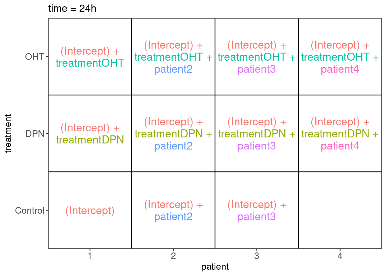ModelMatrix::VisualizeDesign(colData(se),~ time*treatment + patient)$plotlist

## $`time = 24h`

## 
## $`time = 48h`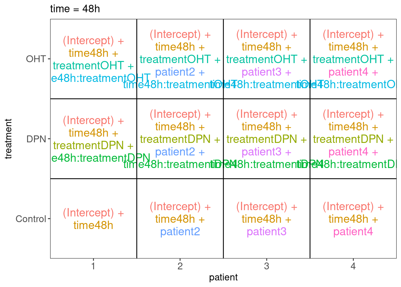

2.3 Filtering

keep <- filterByExpr(dge,design)
table(keep)

## keep
## FALSE  TRUE 
## 46629 16564

dge <- dge[keep, , keep.lib.sizes=FALSE]

2.4 Normalisation

dge <- calcNormFactors(dge)
dge$samples

2.5 Data exploration

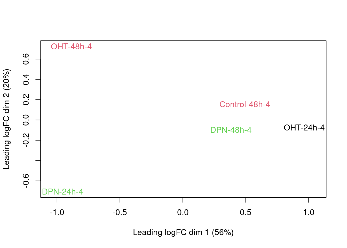
An MDS plot shows the leading fold changes (differential expression) between the 23 samples.

plotMDS(dge,labels=paste(colData(se)$treatment,colData(se)$time,colData(se)$patient,sep="-"),col=as.double(colData(se)$treatment))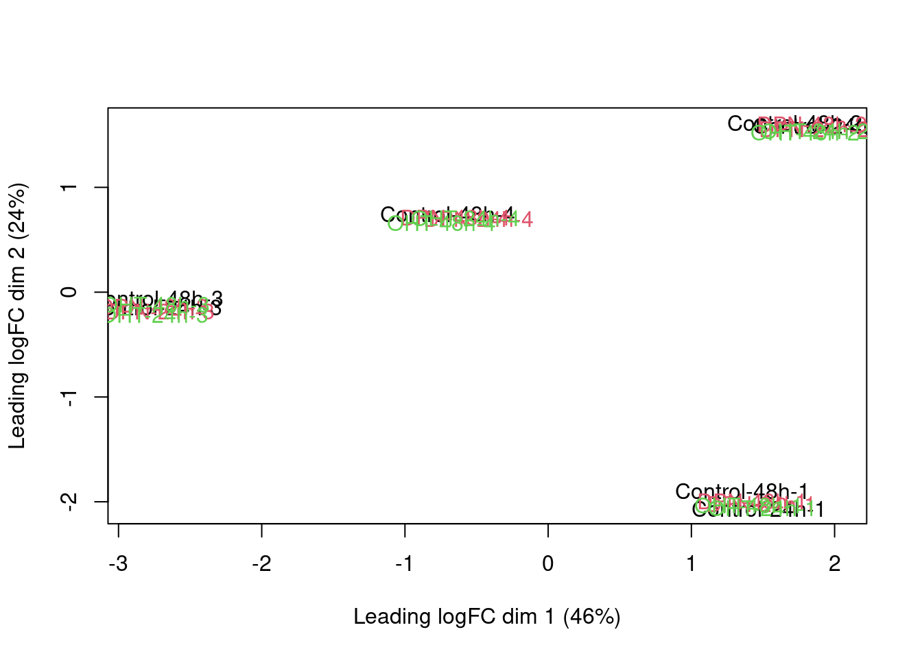

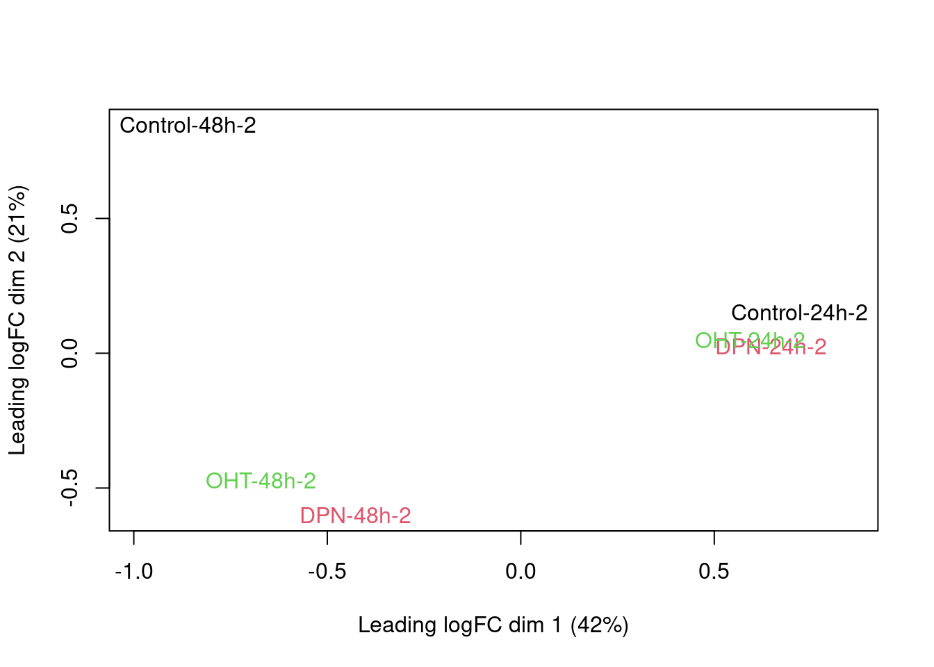
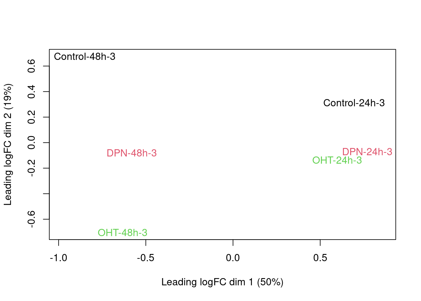
There is a very strong patient effect! To further assess the treatment effects we can make MDS plots per patient

for (i in 1:4)
plotMDS(dge[,colData(se)$patient==i], col=as.double(colData(se)$treatment)[colData(se)$patient==i],
labels=paste(colData(se)$treatment[colData(se)$patient==i],
             colData(se)$time[colData(se)$patient==i],
             colData(se)$patient,sep="-")[colData(se)$patient==i])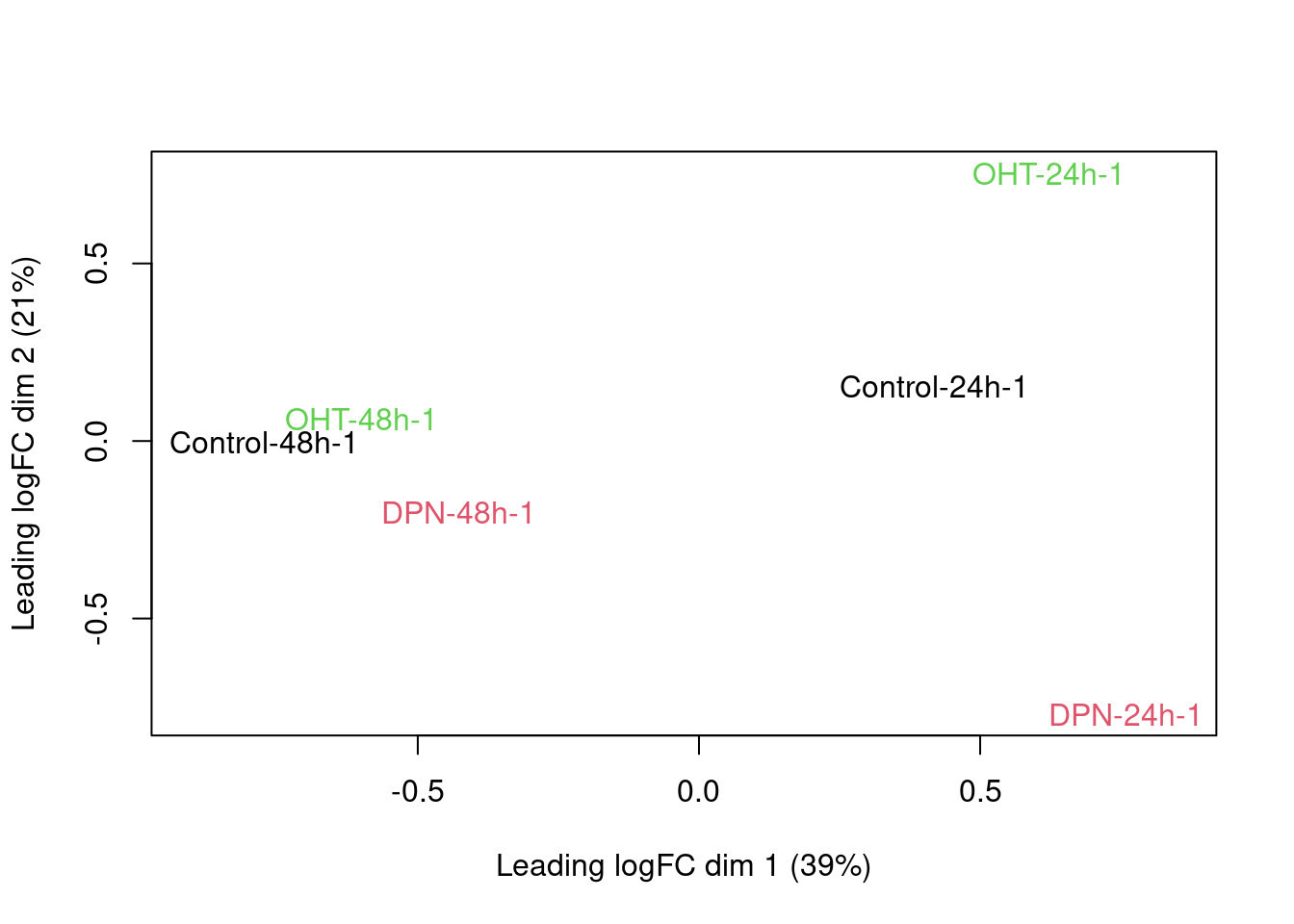

2.6 Parameter estimation

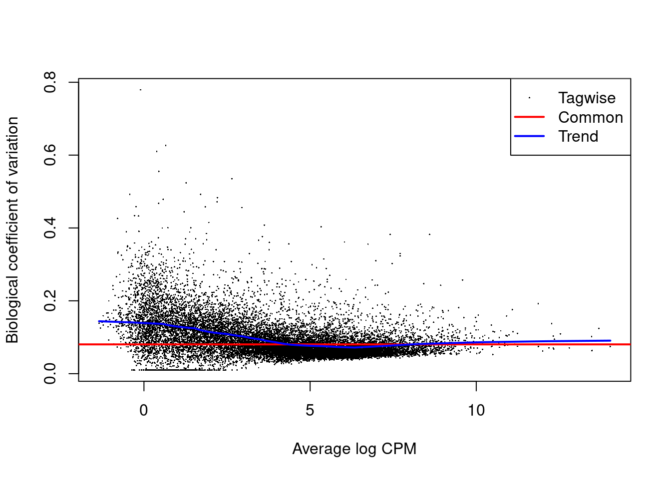
We will use the default Quasi likelihood approach of edgeR.

For quasi-likelihood we do not specify the full distribution, only the first two moments: the mean and the variance, which is sufficient to do inference on the mean.

\[ \left\{ \begin{array}{lcl} E[y_{ig}\vert \mathbf{x}_{ig}]&=&\mu_{ig}\\ log(\mu_{ig})&=&\eta_{ig}\\ \eta_{ig}&=&\beta_0 + \beta_{t2} x_{t2,i} + \beta_{DPN} x_{DPN,i} + \beta_\text{DPN:t2} x_{DPN,i}x_{t2,i} \\ && \quad + \beta_{OHT}x_{OHT,i} + \beta_\text{OHT:t2} x_{OHT,i}x_{t2,i} \\ && \quad + \beta_{p2}x_{p2,i} + \beta_{p3}x_{p3,i} + \beta_{p4}x_{p4,i}\ + \log N_i\\ \text{Var}[y_{ig}\vert \mathbf{x}_{ig}]&=&\sigma^2_g\left(\mu_{ig}+\phi\mu_{ig}^2\right) \end{array}\right. \]

with \(\sigma^2_g\) an additional dispersion parameter the scales the negative binomial variance function, \(x_{DPN,i}\), \(x_{DPN,i}\), \(x_{t2,i}\), \(x_{p.,i}\) dummy variables that is 1 if cell line was treated with DPN, OHT, incubated for 48 h, from patient \(p.\), respectively and is 0 otherwise, and, \(\log{N}_i\) a normalisation offset to correct for sequencing depth. Note, that \(\beta_{DPN}\) is the main effect for the DPN treatment, and corresponds to the average log fold change between treated and control mice after 24h. The interaction \(\beta_\text{DPN:t2}\) can be interpreted as the average change in log2 FC between DPN treated and control cell lines at the late and early timepoint. The researchers are also interested in a assessing third contrast: the effect of the DPN treatment at the late time point.

\[ \log_2\text{FC}^\text{48h}_\text{DPN - C}= \beta_{DPN}+\beta_{DPN,t2}\]

For the OHT treatment we will assess similar contrasts.

\[ \log_2\text{FC}^\text{24h}_\text{OHT - C}= \beta_{OHT}\] \[ \log_2\text{FC}^\text{48h}_\text{OHT - C}= \beta_{OHT}+\beta_{OHT,t2}\] \[ \log_2\text{FC}^\text{48h}_\text{OHT - C} -\log_2\text{FC}^\text{24h}_\text{OHT - C}= \beta_{OHT,t2} \]

Finally, we also have to assess if there is a difference between DPN and OHT treatment

\[ \log_2\text{FC}^\text{24h}_\text{OHT - DPN}= \beta_{OHT} - \beta_{DPN}\] \[ \log_2\text{FC}^\text{48h}_\text{OHT - C}= \beta_{OHT}+\beta_{OHT,t2} - \beta_{DPN} - \beta_{DPN,t2} \]

\[ \log_2\text{FC}^\text{48h}_\text{OHT - DPN} -\log_2\text{FC}^\text{24h}_\text{OHT - DPN}= \beta_{OHT,t2} - \beta_{DPN,t2} \]

dge <- estimateDisp(dge, design)  
plotBCV(dge)

The quasi-negative binomial model can be fitted using the function glmQLFit

fit <- glmQLFit(dge,design)

2.7 Contrasts

We now implement all 9 contrasts of interest

L <- msqrob2::makeContrast(
    c("treatmentDPN = 0",
      "treatmentOHT = 0",
      "treatmentOHT - treatmentDPN = 0", 
      "treatmentDPN + time48h:treatmentDPN = 0",
      "treatmentOHT + time48h:treatmentOHT = 0",
      "treatmentOHT + time48h:treatmentOHT - treatmentDPN - time48h:treatmentDPN = 0", 
      "time48h:treatmentDPN = 0", 
      "time48h:treatmentOHT = 0", 
      "time48h:treatmentOHT - time48h:treatmentDPN = 0"),
    parameterNames = colnames(design))
L

##                      treatmentDPN treatmentOHT treatmentOHT - treatmentDPN
## (Intercept)                     0            0                           0
## time48h                         0            0                           0
## treatmentDPN                    1            0                          -1
## treatmentOHT                    0            1                           1
## patient2                        0            0                           0
## patient3                        0            0                           0
## patient4                        0            0                           0
## time48h:treatmentDPN            0            0                           0
## time48h:treatmentOHT            0            0                           0
##                      treatmentDPN + time48h:treatmentDPN
## (Intercept)                                            0
## time48h                                                0
## treatmentDPN                                           1
## treatmentOHT                                           0
## patient2                                               0
## patient3                                               0
## patient4                                               0
## time48h:treatmentDPN                                   1
## time48h:treatmentOHT                                   0
##                      treatmentOHT + time48h:treatmentOHT
## (Intercept)                                            0
## time48h                                                0
## treatmentDPN                                           0
## treatmentOHT                                           1
## patient2                                               0
## patient3                                               0
## patient4                                               0
## time48h:treatmentDPN                                   0
## time48h:treatmentOHT                                   1
##                      treatmentOHT + time48h:treatmentOHT - treatmentDPN - time48h:treatmentDPN
## (Intercept)                                                                                  0
## time48h                                                                                      0
## treatmentDPN                                                                                -1
## treatmentOHT                                                                                 1
## patient2                                                                                     0
## patient3                                                                                     0
## patient4                                                                                     0
## time48h:treatmentDPN                                                                        -1
## time48h:treatmentOHT                                                                         1
##                      time48h:treatmentDPN time48h:treatmentOHT
## (Intercept)                             0                    0
## time48h                                 0                    0
## treatmentDPN                            0                    0
## treatmentOHT                            0                    0
## patient2                                0                    0
## patient3                                0                    0
## patient4                                0                    0
## time48h:treatmentDPN                    1                    0
## time48h:treatmentOHT                    0                    1
##                      time48h:treatmentOHT - time48h:treatmentDPN
## (Intercept)                                                    0
## time48h                                                        0
## treatmentDPN                                                   0
## treatmentOHT                                                   0
## patient2                                                       0
## patient3                                                       0
## patient4                                                       0
## time48h:treatmentDPN                                          -1
## time48h:treatmentOHT                                           1

2.8 Tests

We have to perform a quasi- F-test for each contrast. The quasi F-test involves fitting a different model for each contrast so that we can compare the full model with a reduced model that implies that one specific contrast is zero.

Because we estimated the additional dispersion parameter \(\sigma^2_g\) using a sum of squared deviance residuals:

i.e.  \[e_{i,d} = 2 (l_i(y_i,y_i) - l_i(\mu_i,y_i)\] and

\[ \hat \sigma_g^2 = \frac{\sum_{i=1}^n e_{i,d}^2}{n-p} = \frac{2\left[l(\mathbf{y},\mathbf{y}) - l(\boldsymbol{\mu},\mathbf{y})\right]}{n-p} \]

With edgeR we will then further adopt empirical Bayes to borrow strength across genes to stabilise the parameter estimator, which will also increase the degrees if this gene wise dispersion parameter estimator which we refer to as \(df_\text{res}^{EB}\).

We can use a quasi F -test that can also correct for the degrees of freedom that have been used to estimate mean model parameters and the residual degrees of freedom that were available for estimating the additional dispersion parameter. The quasi F test will thus perform better in a small sample setting. It is defined as:

\[ F = \frac{\frac{LRT_\text{g, full - reduced}}{df_{LRT}}}{\sigma^2_g} \]

which follows an F - distribution with \(df_{LRT}\) degrees of freedom in the nominator and \(df_{res}^{EB}\) degrees of freedom in the denominator under the null hypothesis that the full and reduced model are equivalent and that the assessed contrasts are thus equal to zero. Indeed, the dispersion estimator in the denominator follows a scaled \(\chi^2\) distribution with \(df_{res}^{EB}\) degrees of freedom.

We perform all tests and loop over the columns of L for this purpose.

testsF <- apply(L, 2, function(fit,contrast) 
    glmQLFTest(fit,contrast=contrast), 
    fit = fit)
topTablesF<- lapply(testsF, topTags, n=nrow(dge))

sapply(topTablesF, function(x) sum(x$table$FDR <0.05))

##                                                              treatmentDPN 
##                                                                         0 
##                                                              treatmentOHT 
##                                                                         0 
##                                               treatmentOHT - treatmentDPN 
##                                                                         0 
##                                       treatmentDPN + time48h:treatmentDPN 
##                                                                         5 
##                                       treatmentOHT + time48h:treatmentOHT 
##                                                                        11 
## treatmentOHT + time48h:treatmentOHT - treatmentDPN - time48h:treatmentDPN 
##                                                                         0 
##                                                      time48h:treatmentDPN 
##                                                                         0 
##                                                      time48h:treatmentOHT 
##                                                                         0 
##                               time48h:treatmentOHT - time48h:treatmentDPN 
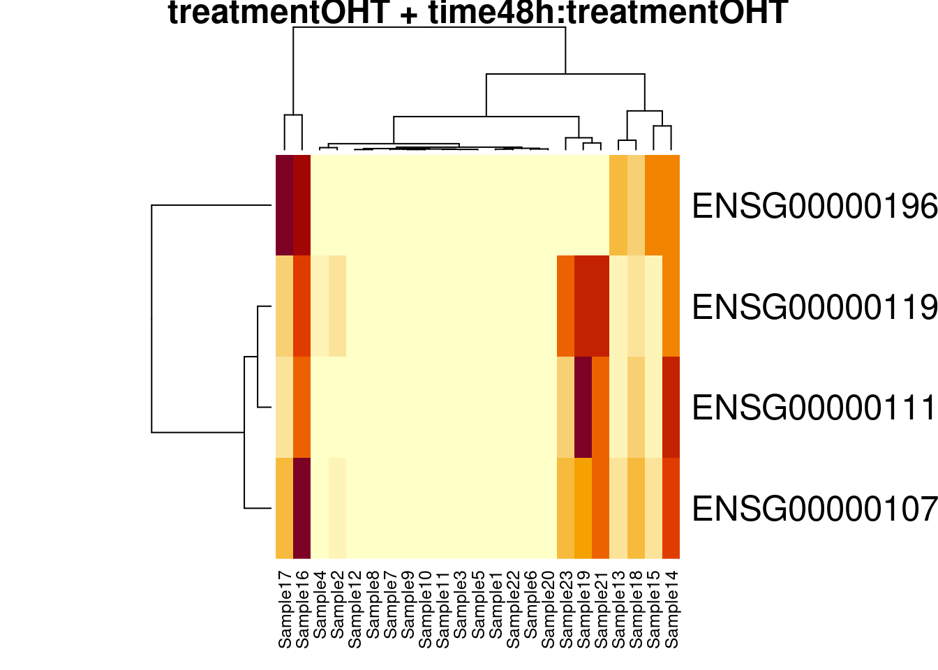
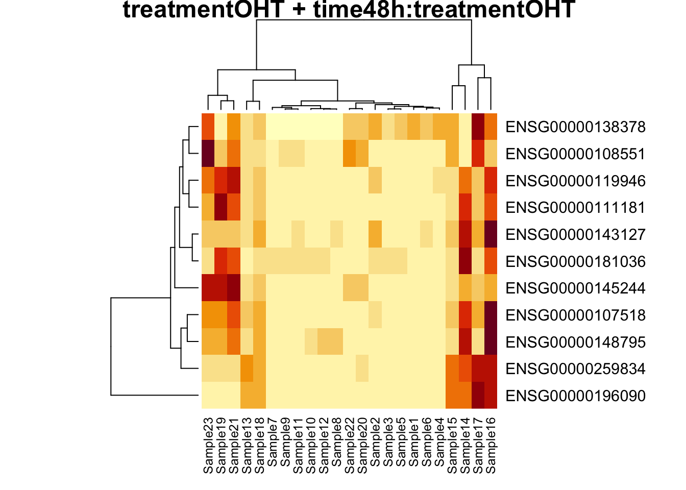
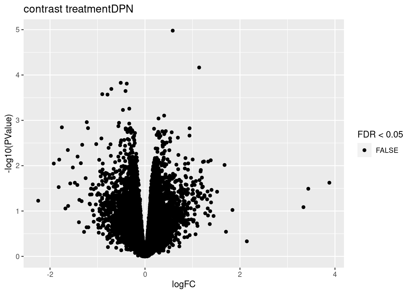
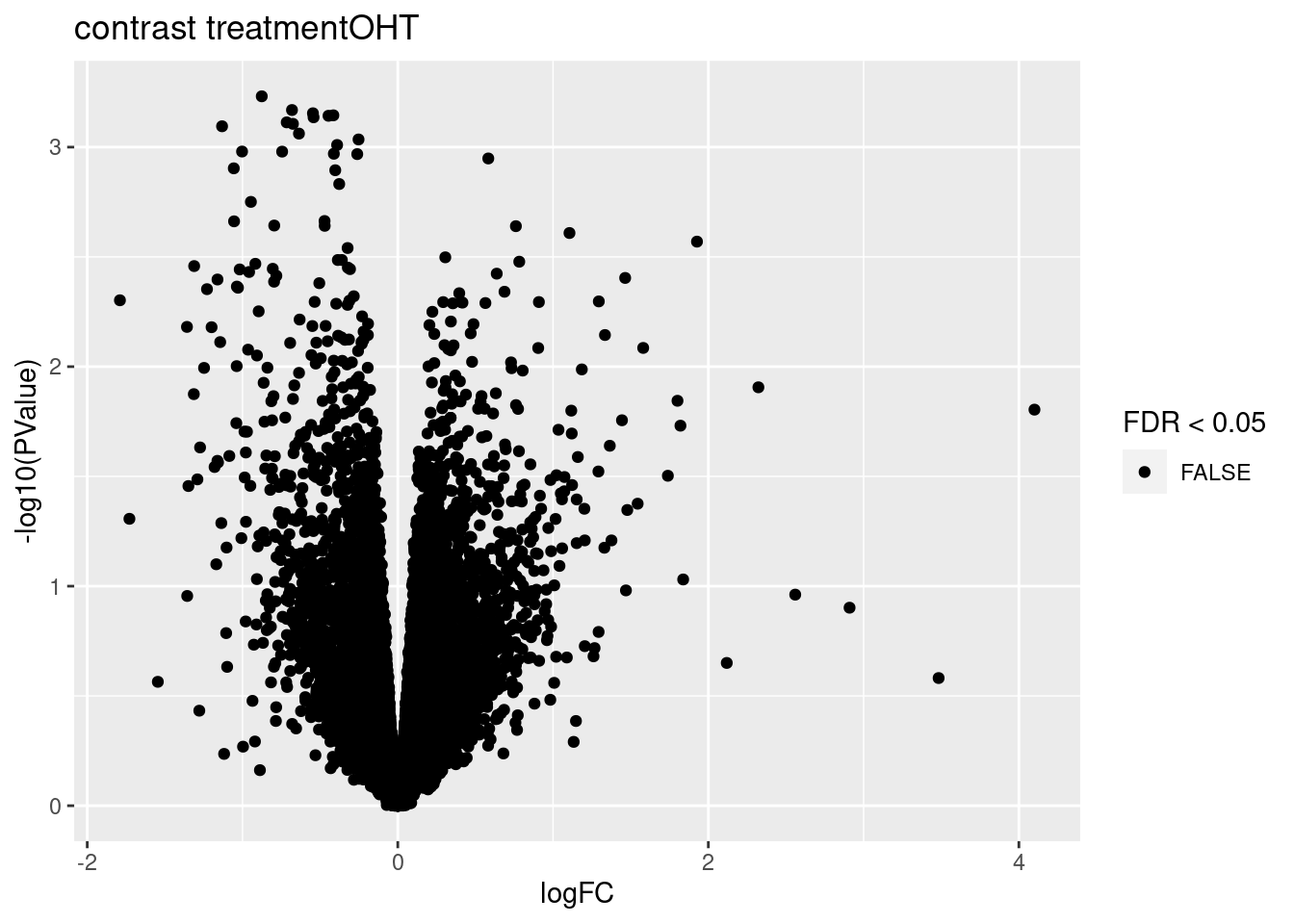
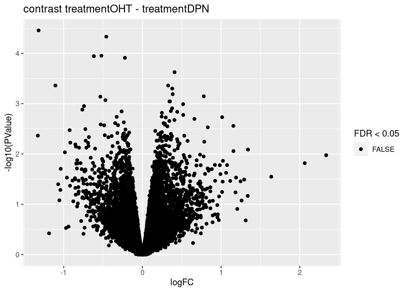
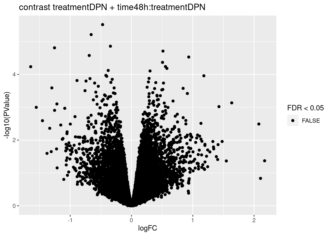
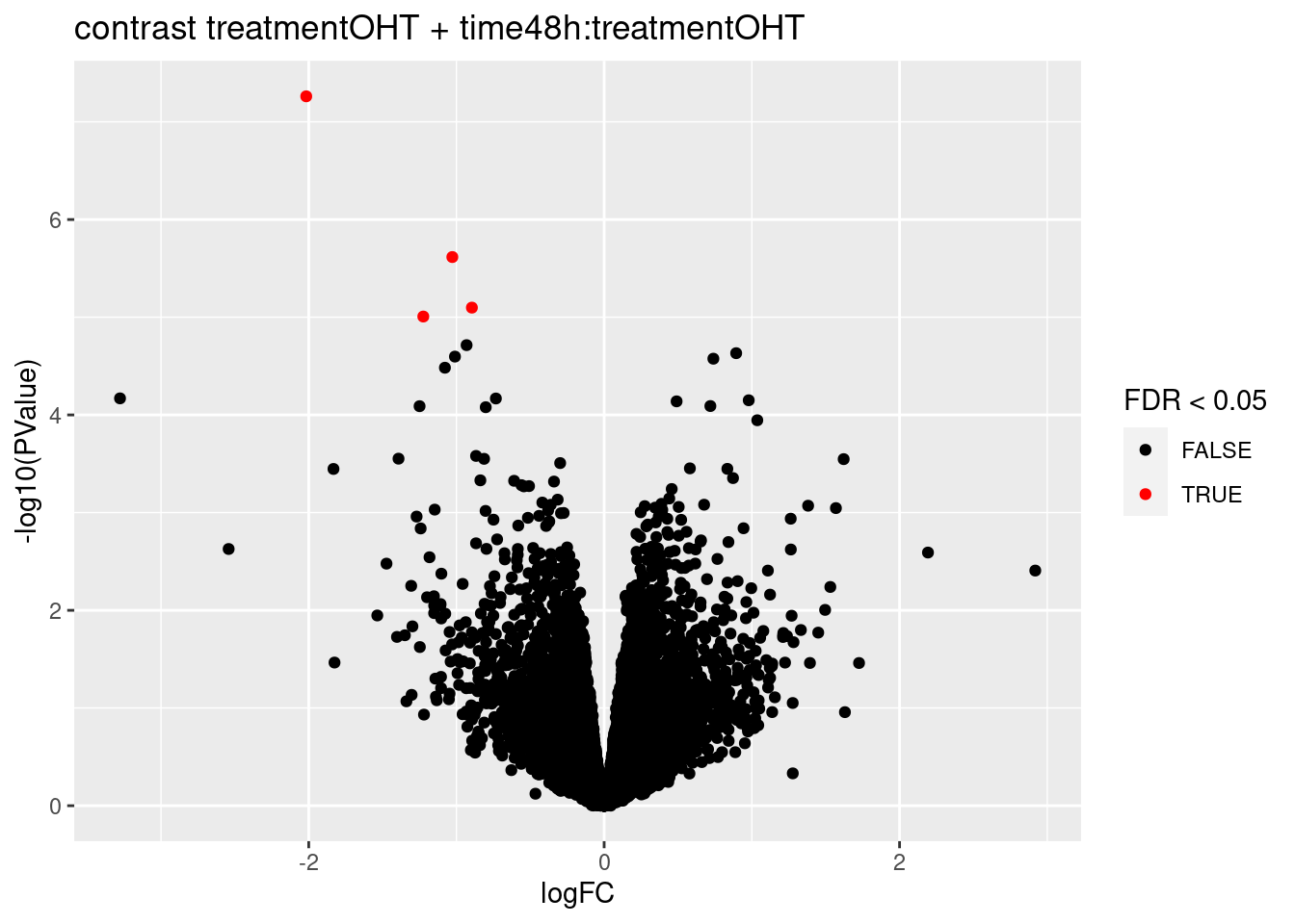
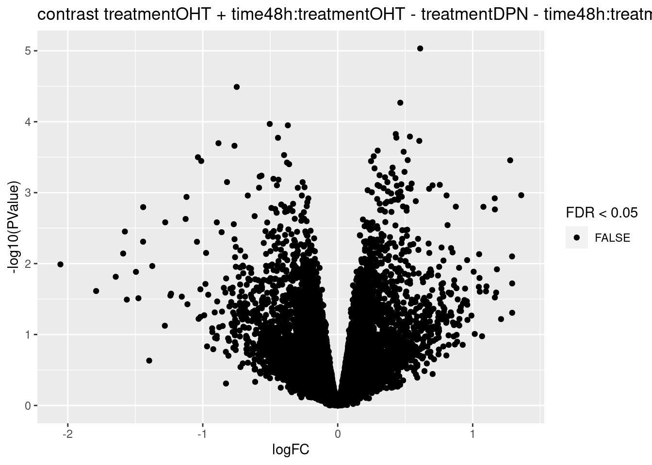
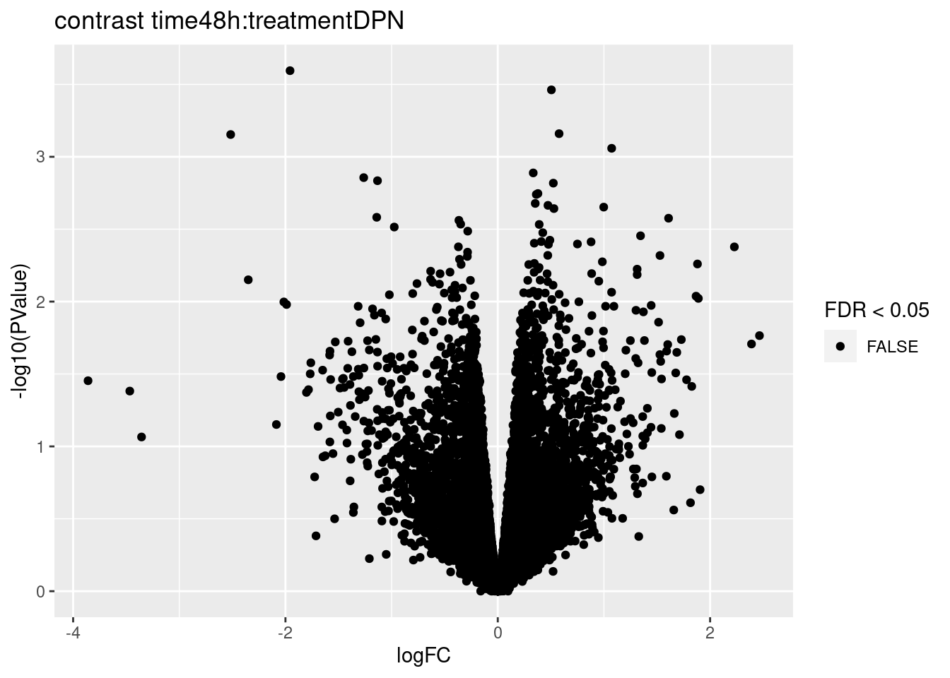
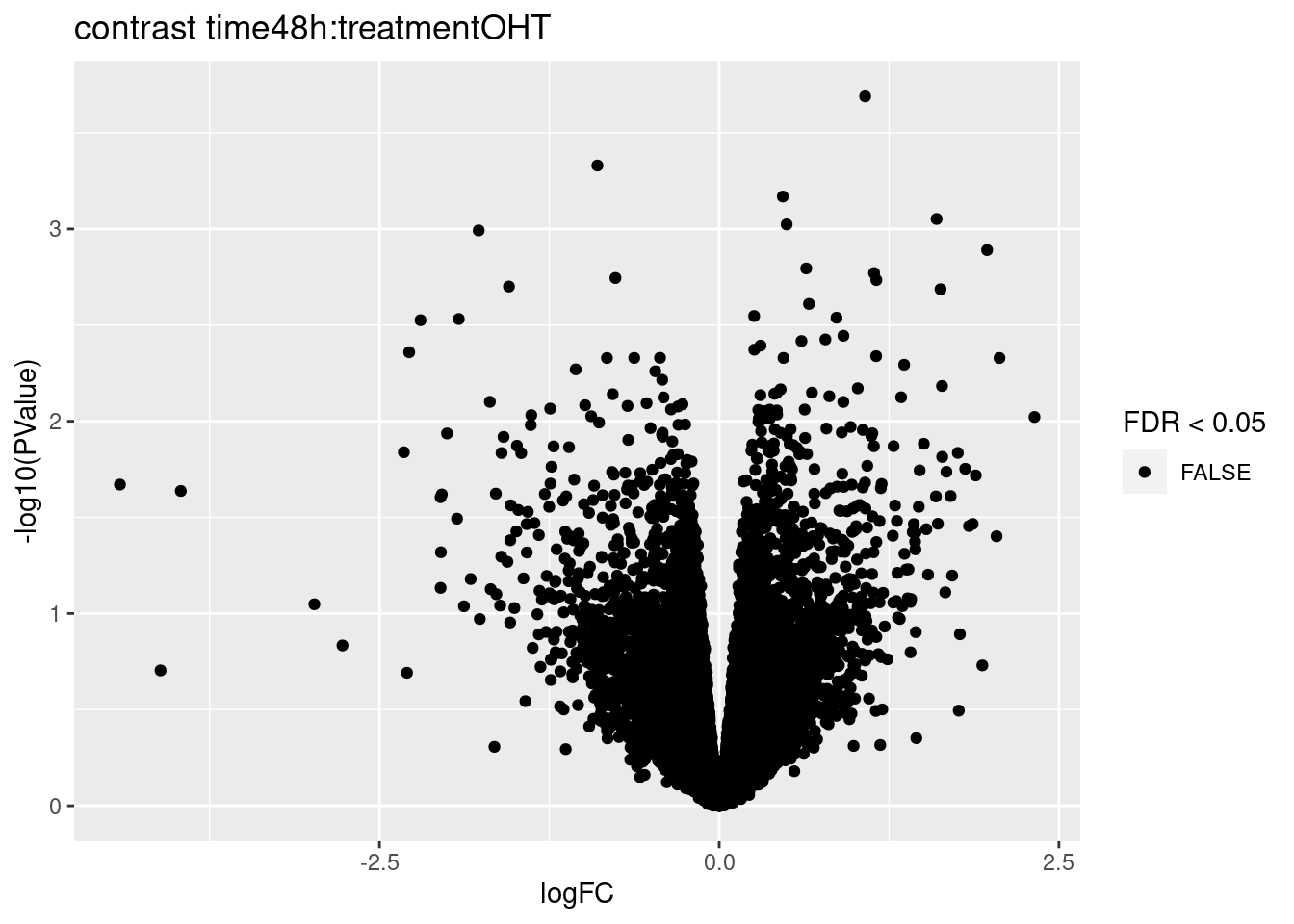
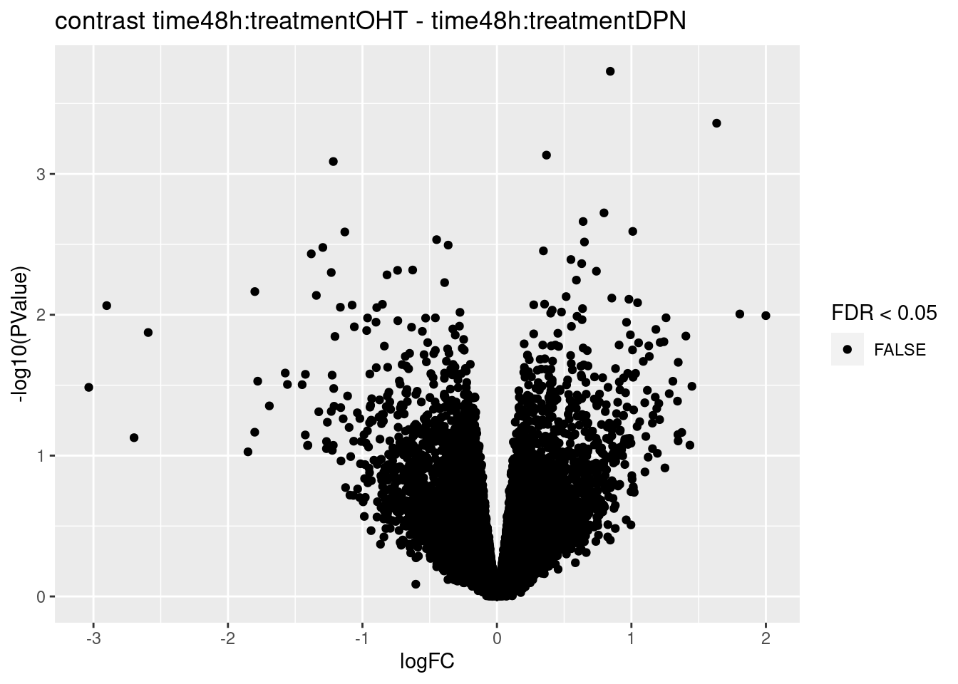
##                                                                         0

We only find significant fold changes for very few genes between OHT and the control treatment at the late time point. We also did not find significant interactions.

3 Plots

3.1 Volcano plots

for (i in 1:ncol(L))
{
   volcano<- ggplot(topTablesF[[i]]$table,aes(x=logFC,y=-log10(PValue),color=FDR < 0.05)) + geom_point() + scale_color_manual(values=c("black","red")) + ggtitle(paste("contrast",names(topTablesF)[i]))
print(volcano)
}

3.2 Histograms of p-values

histsP <- lapply(topTablesF, function(x) 
    x$table %>% 
        ggplot(aes(x=PValue)) + 
        geom_histogram(breaks =seq(0,1,.1) ,col=1)
    )
    
for (i in 1:ncol(L)) 
    histsP[[i]] <- histsP[[i]] +
    ggtitle(paste("contrast",names(topTablesF)[i]))
histsP

## $treatmentDPN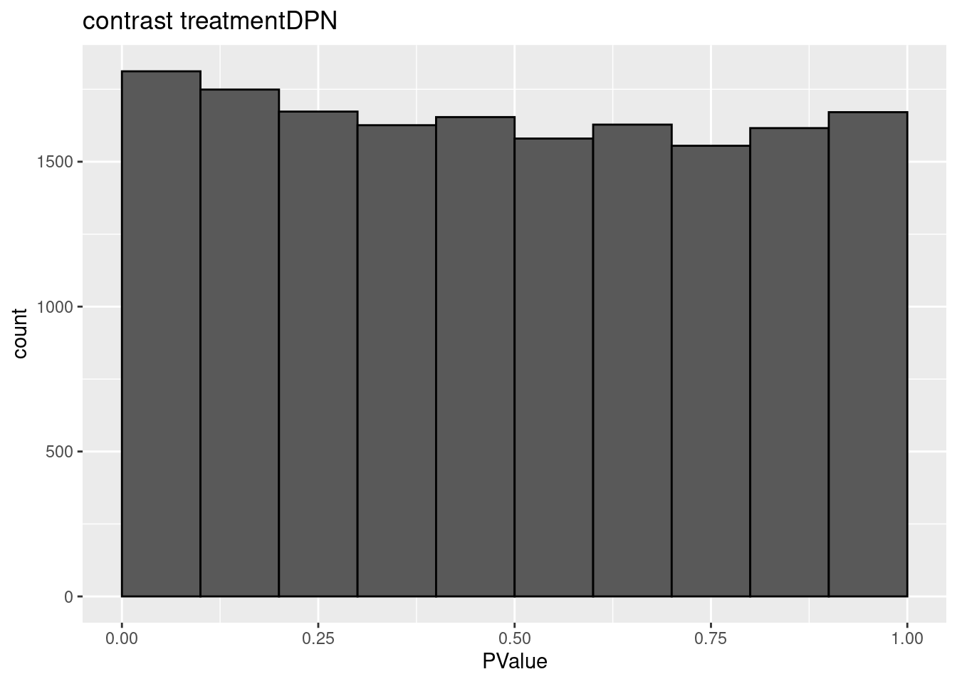

## 
## $treatmentOHT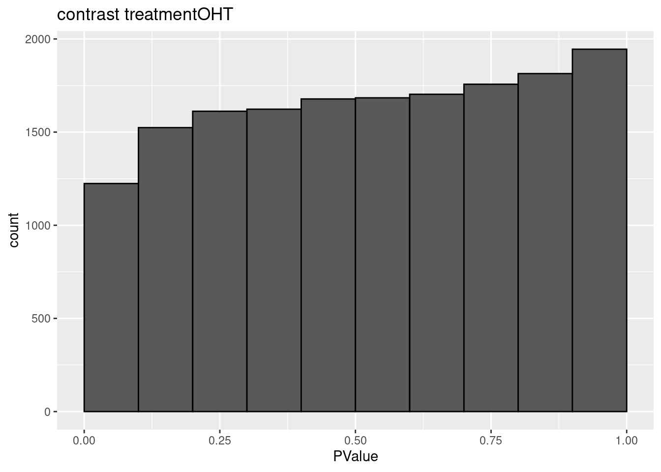

## 
## $`treatmentOHT - treatmentDPN`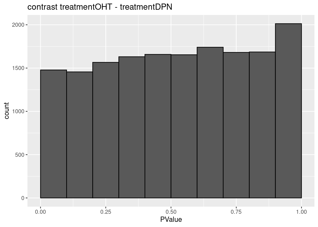

## 
## $`treatmentDPN + time48h:treatmentDPN`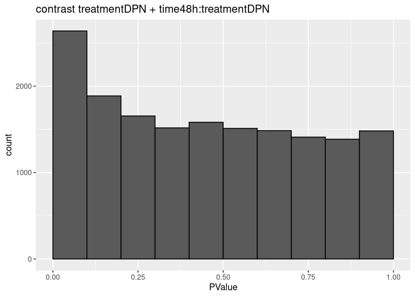

## 
## $`treatmentOHT + time48h:treatmentOHT`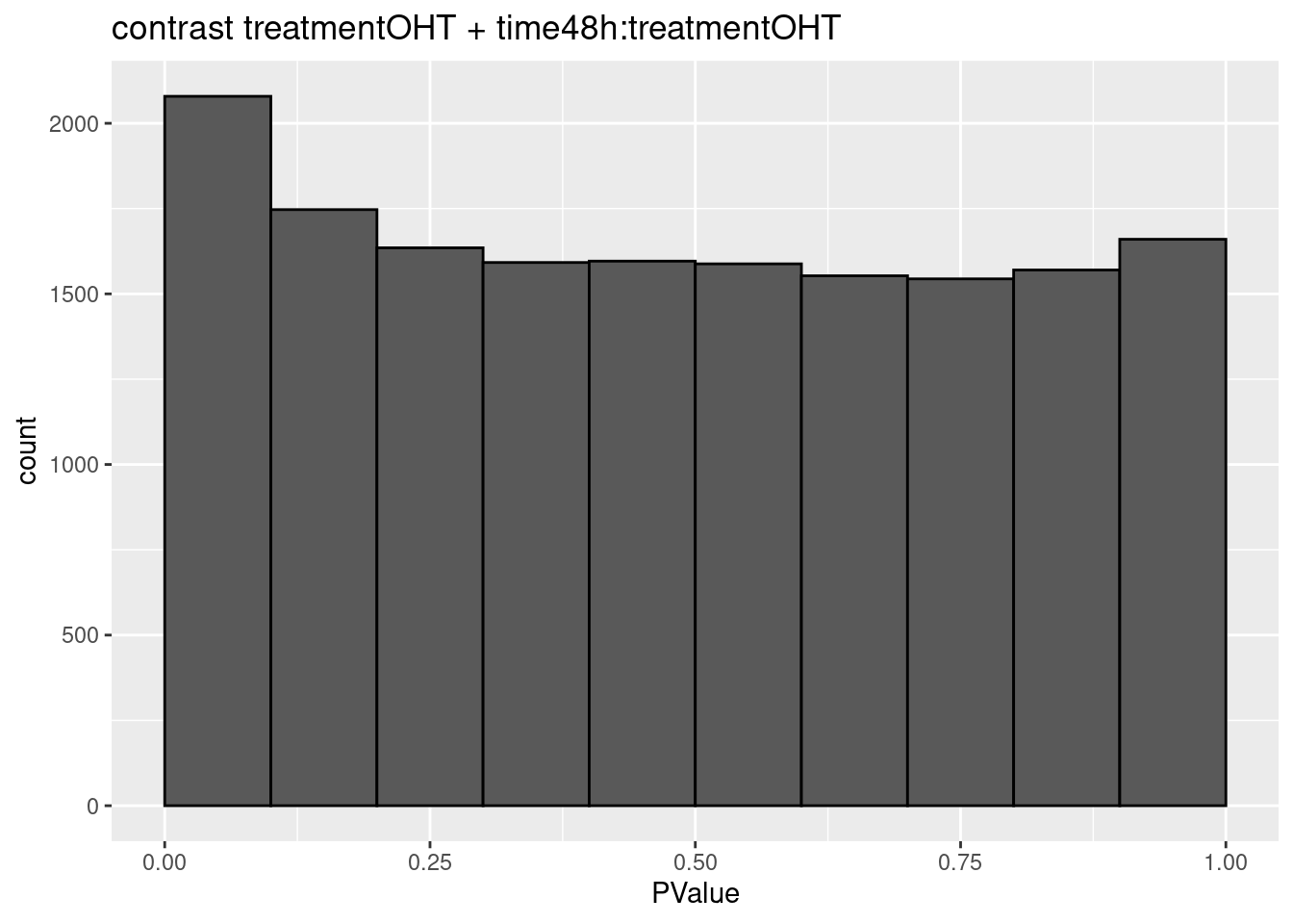

## 
## $`treatmentOHT + time48h:treatmentOHT - treatmentDPN - time48h:treatmentDPN`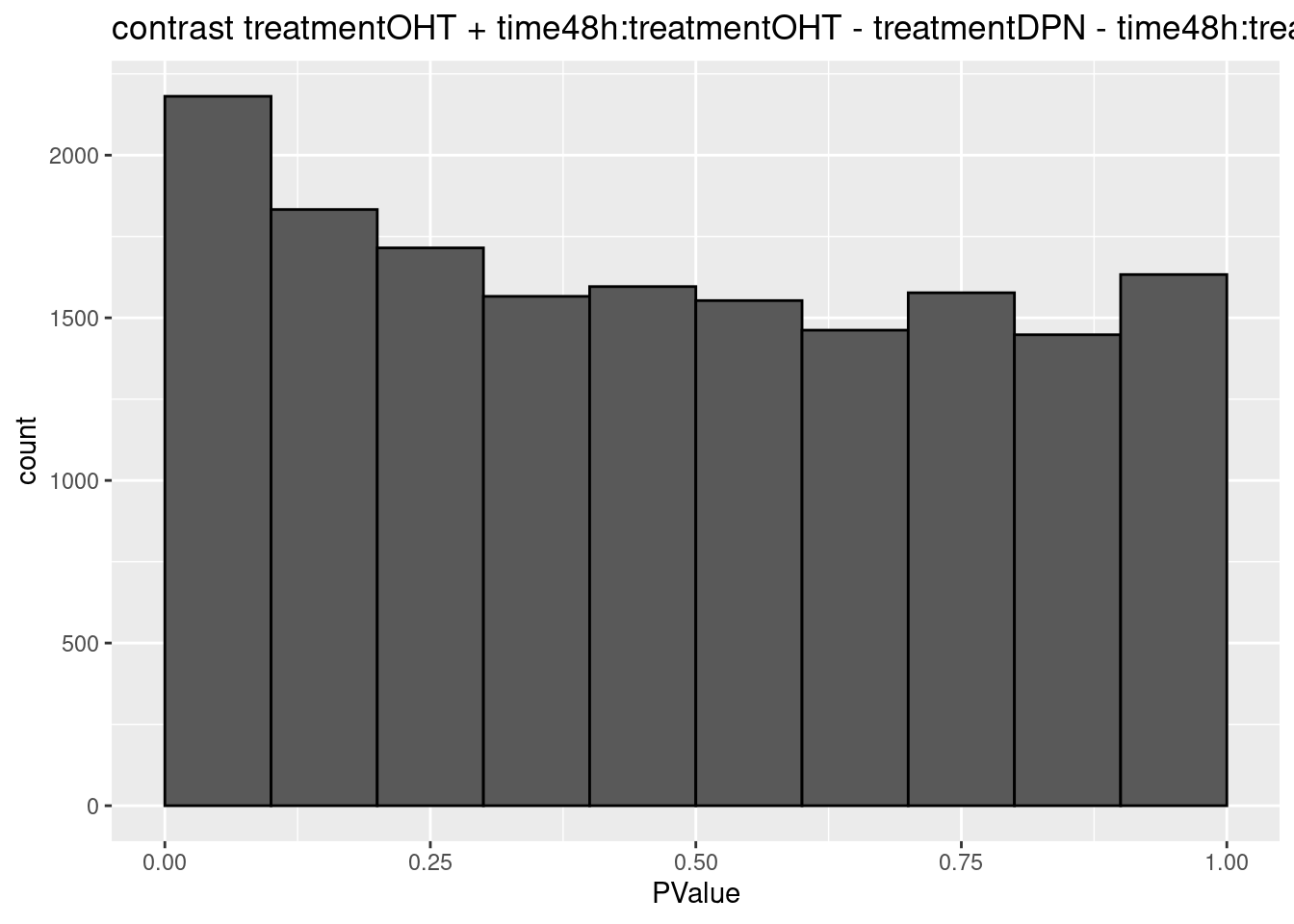

## 
## $`time48h:treatmentDPN`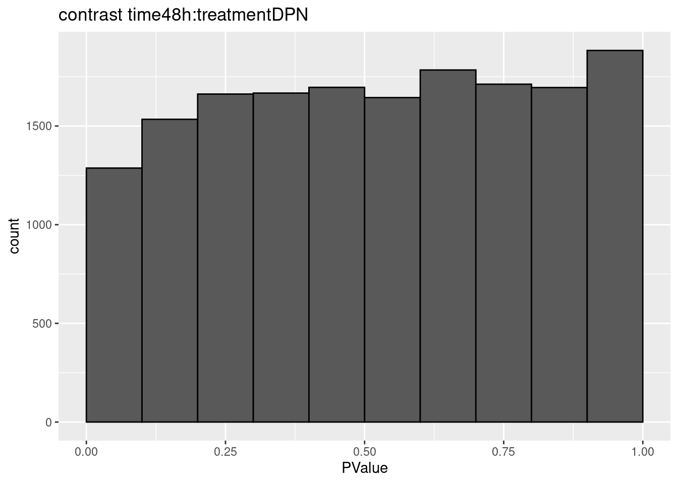

## 
## $`time48h:treatmentOHT`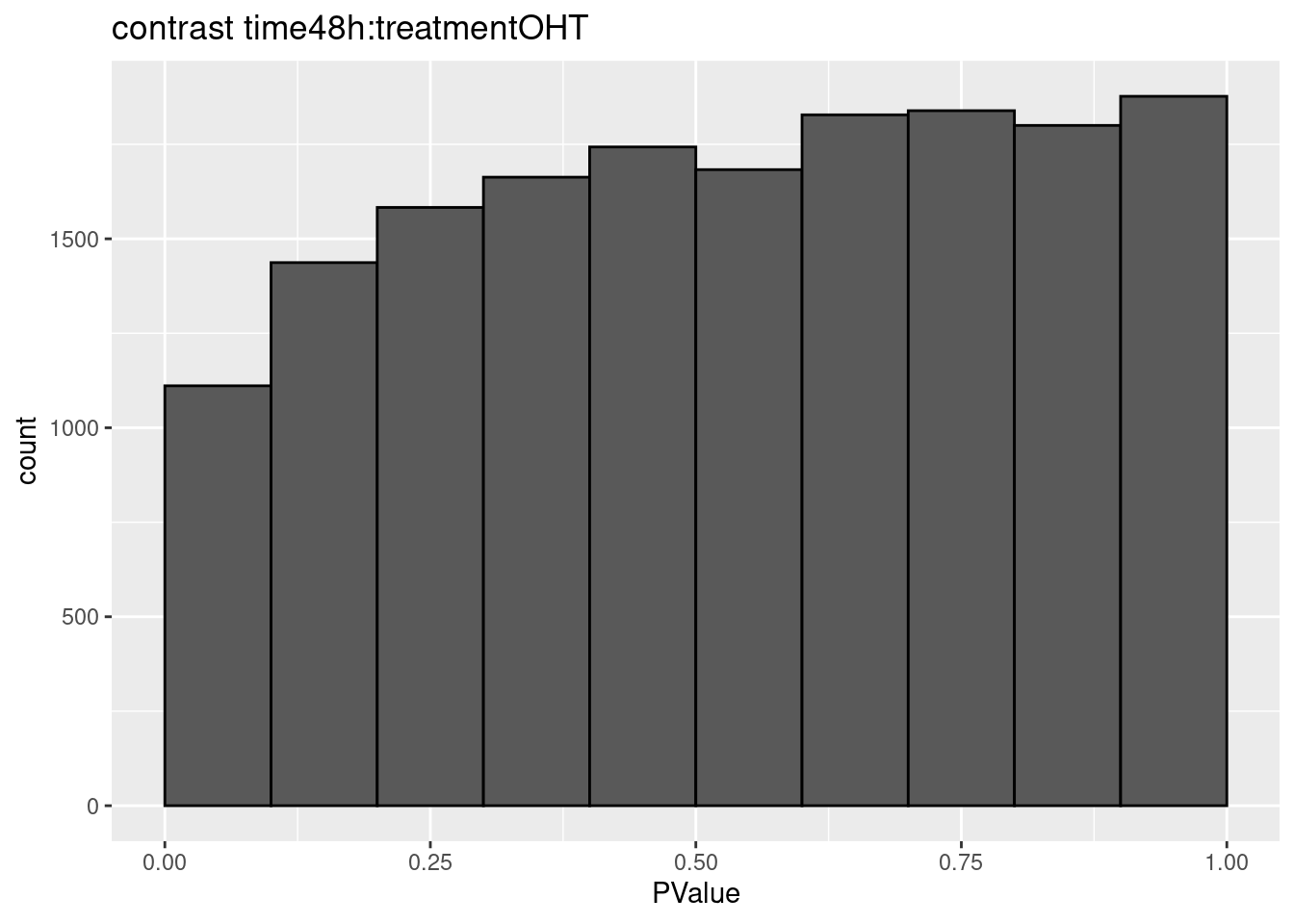

## 
## $`time48h:treatmentOHT - time48h:treatmentDPN`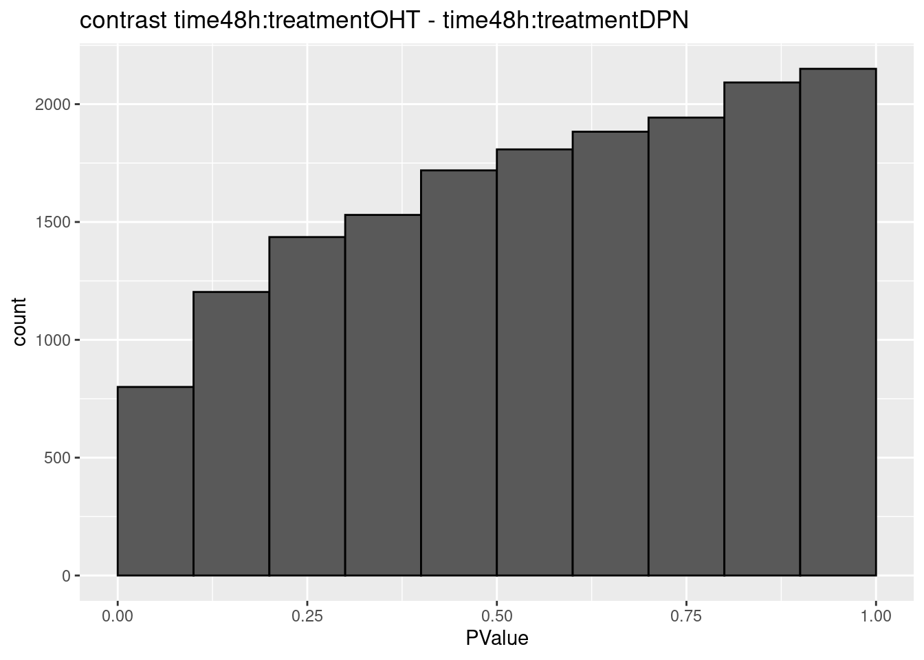

3.3 heatmaps

for (i in 1:ncol(L))
{
    sigID <- topTablesF[[i]]$table %>% 
        filter(FDR<0.05) %>% 
        rownames
    if (length(sigID)>0)
        heatmap(dge$counts[sigID,], main = colnames(L)[i], cex.main=.2)
}

4 EdgeR traditional

fitGlm <- glmFit(dge,design)
testLRT2 <- apply(L, 2, function(fit,contrast) 
    glmLRT(fit,contrast=contrast), 
    fit = fitGlm)
topTablesLRT2 <- lapply(testLRT2, topTags, n=nrow(dge))
sapply(topTablesLRT2, function(x) sum(x$table$FDR <0.05))

##                                                              treatmentDPN 
##                                                                         2 
##                                                              treatmentOHT 
##                                                                         0 
##                                               treatmentOHT - treatmentDPN 
##                                                                         4 
##                                       treatmentDPN + time48h:treatmentDPN 
##                                                                        64 
##                                       treatmentOHT + time48h:treatmentOHT 
##                                                                        23 
## treatmentOHT + time48h:treatmentOHT - treatmentDPN - time48h:treatmentDPN 
##                                                                        11 
##                                                      time48h:treatmentDPN 
##                                                                         0 
##                                                      time48h:treatmentOHT 
##                                                                         0 
##                               time48h:treatmentOHT - time48h:treatmentDPN 
##                                                                         0

We find more genes for the traditional edgeR workflow, however, it is known that this workflow is often too liberal.