Airway: DE analysis based on transcript counts and DESeq2

1 Background

The data used in this workflow comes from an RNA-seq experiment where airway smooth muscle cells were treated with dexamethasone, a synthetic glucocorticoid steroid with anti-inflammatory effects (Himes et al. 2014). Glucocorticoids are used, for example, by people with asthma to reduce inflammation of the airways. In the experiment, four human airway smooth muscle cell lines were treated with 1 micromolar dexamethasone for 18 hours. For each of the four cell lines, we have a treated and an untreated sample. For more description of the experiment see the article, PubMed entry 24926665, and for raw data see the GEO entry GSE52778.

Many parts of this tutorial are based on parts of a published RNA-seq workflow available via Love et al. 2015 F1000Research and as a Bioconductor package and on Charlotte Soneson’s material from the bss2019 workshop.

2 Data

We will use the salmon quantification files here. This is a lightweight transcript level mapper.

2.1 Meta data

As before, we will retrieve the meta data by linking the SRA files to the meta data on GEO.

library(edgeR)

## Loading required package: limma

library(tidyverse)

## ── Attaching core tidyverse packages ──────────────────────── tidyverse 2.0.0 ──
## ✔ dplyr     1.1.4     ✔ readr     2.1.5
## ✔ forcats   1.0.0     ✔ stringr   1.5.1
## ✔ ggplot2   3.5.1     ✔ tibble    3.2.1
## ✔ lubridate 1.9.3     ✔ tidyr     1.3.1
## ✔ purrr     1.0.2

## ── Conflicts ────────────────────────────────────────── tidyverse_conflicts() ──
## ✖ dplyr::filter() masks stats::filter()
## ✖ dplyr::lag()    masks stats::lag()
## ℹ Use the conflicted package (<http://conflicted.r-lib.org/>) to force all conflicts to become errors

library(GEOquery)

## Loading required package: Biobase
## Loading required package: BiocGenerics
## 
## Attaching package: 'BiocGenerics'
## 
## The following objects are masked from 'package:lubridate':
## 
##     intersect, setdiff, union
## 
## The following objects are masked from 'package:dplyr':
## 
##     combine, intersect, setdiff, union
## 
## The following object is masked from 'package:limma':
## 
##     plotMA
## 
## The following objects are masked from 'package:stats':
## 
##     IQR, mad, sd, var, xtabs
## 
## The following objects are masked from 'package:base':
## 
##     anyDuplicated, aperm, append, as.data.frame, basename, cbind,
##     colnames, dirname, do.call, duplicated, eval, evalq, Filter, Find,
##     get, grep, grepl, intersect, is.unsorted, lapply, Map, mapply,
##     match, mget, order, paste, pmax, pmax.int, pmin, pmin.int,
##     Position, rank, rbind, Reduce, rownames, sapply, setdiff, table,
##     tapply, union, unique, unsplit, which.max, which.min
## 
## Welcome to Bioconductor
## 
##     Vignettes contain introductory material; view with
##     'browseVignettes()'. To cite Bioconductor, see
##     'citation("Biobase")', and for packages 'citation("pkgname")'.
## 
## Setting options('download.file.method.GEOquery'='auto')
## Setting options('GEOquery.inmemory.gpl'=FALSE)

download.file("https://github.com/statOmics/SGA/archive/airwaySeqData.zip","SGA-airwaySeqData.zip")
unzip("SGA-airwaySeqData.zip", exdir = "./")

2.1.1 GEO data

gse<-getGEO("GSE52778")

## Found 1 file(s)

## GSE52778_series_matrix.txt.gz

pdata<-pData(gse[[1]])
pdata$SampleName<-rownames(pdata) %>% as.factor
head(pdata)[1:6,]

2.1.2 SRA info

Download SRA info. To link sample info to info sequencing: Go to corresponding SRA page and save the information via the “Send to: File button” This file can also be used to make a script to download sequencing files from the web. Note that sra files can be converted to fastq files via the fastq-dump function of the sra-tools.

File is also available on course website.

sraInfo<-read.csv("https://raw.githubusercontent.com/statOmics/SGA/airwaySeqData/SraRunInfo.csv")
sraInfo$SampleName <- as.factor(sraInfo$SampleName)
levels(pdata$SampleName)==levels(sraInfo$SampleName)

##  [1] TRUE TRUE TRUE TRUE TRUE TRUE TRUE TRUE TRUE TRUE TRUE TRUE TRUE TRUE TRUE
## [16] TRUE

SampleNames are can be linked.

pdata<-merge(pdata,sraInfo,by="SampleName")
pdata$Run

##  [1] "SRR1039508" "SRR1039509" "SRR1039510" "SRR1039511" "SRR1039512"
##  [6] "SRR1039513" "SRR1039514" "SRR1039515" "SRR1039516" "SRR1039517"
## [11] "SRR1039518" "SRR1039519" "SRR1039520" "SRR1039521" "SRR1039522"
## [16] "SRR1039523"

We do not have the Albuterol samples

rownames(pdata) <- pdata$Run
pdata <- pdata[-grep("Albuterol",pdata[,"treatment:ch1"]),]
pdata[,grep(":ch1",colnames(pdata))]

pdata$cellLine <- pdata[, grep("cell line:ch1", colnames(pdata))] %>%
  as.factor
pdata$treatment<-pdata[, grep("treatment:ch1", colnames(pdata))] %>%
  as.factor
pdata$treatment<-relevel(pdata$treatment, "Untreated")

2.2 Alignment-free transcript quantification

Software such as kallisto [@Bray2016Near], Salmon [@Patro2017Salmon] and Sailfish [@Patro2014Sailfish], as well as other transcript quantification methods like Cufflinks [@Trapnell2010Cufflinks; @Trapnell2013Cufflinks2] and RSEM [@Li2011RSEM], differ from the counting methods introduced in the previous tutorials in that they provide quantifications (usually both as counts and as TPMs) for each transcript. These can then be summarized on the gene level by adding all values for transcripts from the same gene. A simple way to import results from these packages into R is provided by the tximport and tximeta packages. Here, tximport reads the quantifications into a list of matrices, and tximeta aggregates the information into a SummarizedExperiment object, and also automatically adds additional annotations for the features. Both packages can return quantifications on the transcript level or aggregate them on the gene level. They also calculate average transcript lengths for each gene and each sample, which can be used as offsets to improve the differential expression analysis by accounting for differential isoform usage across samples [@Soneson2015Differential]. aturecounts object

2.2.1 Libraries

suppressPackageStartupMessages({
  if(!"tximeta" %in% installed.packages()[,1]) BiocManager::install("tximeta")
  if(!"org.Hs.eg.db" %in% installed.packages()[,1]) BiocManager::install("org.Hs.eg.db")
  library(tximeta)
  library(org.Hs.eg.db)
  library(SummarizedExperiment)
  library(ggplot2)
  library(tidyverse)
})

2.2.2 Importing Salmon abundance quantification

The code below imports the Salmon quantifications into R using the tximeta package. Note how the transcriptome that was used for the quantification is automatically recognized and used to annotate the resulting data object. In order for this to work, tximeta requires that the output folder structure from Salmon is retained, since it reads information from the associated log files in addition to the quantified abundances themselves. With the addIds() function, we can add additional annotation columns.

## List all quant.sf output files from Salmon
salmonfiles <- paste0("SGA-airwaySeqData/salmon/", pdata$Run, "/quant.sf")
names(salmonfiles) <- pdata$Run
stopifnot(all(file.exists(salmonfiles)))

## Add a column "files" to the metadata table. This table must contain at least
## two columns: "names" and "files"
coldata <- cbind(pdata, files = salmonfiles, stringsAsFactors = FALSE)
coldata$names <- coldata$Run

## Import quantifications on the transcript level
st <- tximeta::tximeta(coldata,importer=read.delim)

## importing quantifications

## 1 2 3 4 5 6 7 8 
## found matching transcriptome:
## [ GENCODE - Homo sapiens - release 29 ]
## loading existing TxDb created: 2022-11-17 14:51:16
## Loading required package: GenomicFeatures
## loading existing transcript ranges created: 2022-11-17 14:51:17

## Summarize quantifications on the gene level
sg <- tximeta::summarizeToGene(st)

## loading existing TxDb created: 2022-11-17 14:51:16
## obtaining transcript-to-gene mapping from database
## loading existing gene ranges created: 2022-11-17 14:51:41
## gene ranges assigned by total range of isoforms, see `assignRanges`
## summarizing abundance
## summarizing counts
## summarizing length

## Add gene symbols
sg <- tximeta::addIds(sg, "SYMBOL", gene = TRUE)

## mapping to new IDs using org.Hs.eg.db
## if all matching IDs are desired, and '1:many mappings' are reported,
## set multiVals='list' to obtain all the matching IDs
## 'select()' returned 1:many mapping between keys and columns

sg

## class: RangedSummarizedExperiment 
## dim: 58294 8 
## metadata(7): tximetaInfo quantInfo ... txdbInfo assignRanges
## assays(3): counts abundance length
## rownames(58294): ENSG00000000003.14 ENSG00000000005.5 ...
##   ENSG00000285993.1 ENSG00000285994.1
## rowData names(3): gene_id tx_ids SYMBOL
## colnames(8): SRR1039508 SRR1039509 ... SRR1039520 SRR1039521
## colData names(101): SampleName title ... treatment names

Note that Salmon returns estimated counts, which are not necessarily integers. They may need to be rounded before they are passed to count-based statistical methods (e.g. DESeq2). This is not necesary for edgeR.

3 DE analysis at the gene level

3.1 Setup count object in edgeR

suppressPackageStartupMessages({
  library(edgeR)
})
dge <- makeDGEList(sg)

3.2 Filtering and normalisation

design <- model.matrix(~treatment+cellLine,data=colData(sg))
keep <- filterByExpr(dge, design)
dge <- dge[keep, ,keep.lib.sizes=FALSE]
dge <- calcNormFactors(dge)

## Warning in calcNormFactors.DGEList(dge): object contains offsets, which take precedence over library
## sizes and norm factors (and which will not be recomputed).

dge$samples

Note, that the recalculation of libsizes and normalisation factors are overruled because we already have calculated user defined offsets.

3.3 Data exploration

One way to reduce dimensionality is the use of multidimensional scaling (MDS). For MDS, we first have to calculate all pairwise distances between our objects (samples in this case), and then create a (typically) two-dimensional representation where these pre-calculated distances are represented as accurately as possible. This means that depending on how the pairwise sample distances are defined, the two-dimensional plot can be very different, and it is important to choose a distance that is suitable for the type of data at hand.

edgeR contains a function plotMDS, which operates on a DGEList object and generates a two-dimensional MDS representation of the samples. The default distance between two samples can be interpreted as the “typical” log fold change between the two samples, for the genes that are most different between them (by default, the top 500 genes, but this can be modified). We generate an MDS plot from the DGEList object dge, coloring by the treatment and using different plot symbols for different cell lines.

colnames(dge) <- paste0(substr(pdata$cellLine,1,3),"_",substr(pdata$treatment,1,3))
plotMDS(dge, top = 500,col=as.double(colData(sg)$cellLine))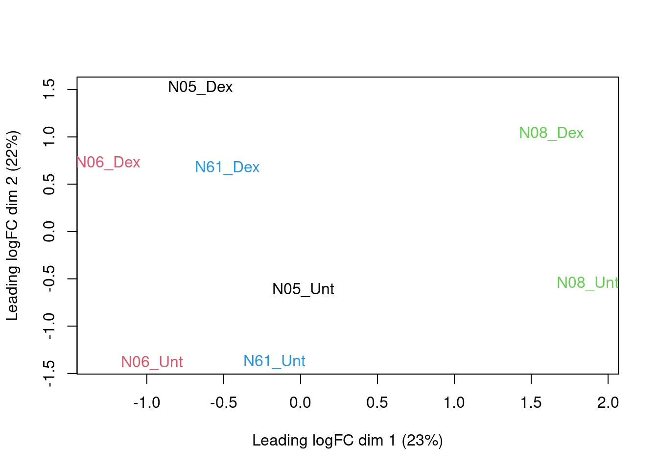

3.4 Model

3.4.1 Estimate the overdispersion.

dge <- estimateDisp(dge, design)
plotBCV(dge)

3.5 Fit the genelevel quasi-NB model.

fit <- glmQLFit(dge, design)
ftest <- glmQLFTest(fit, coef = "treatmentDexamethasone")
ttAll <- topTags(ftest, n = nrow(dge)) # all genes
hist(ttAll$table$PValue)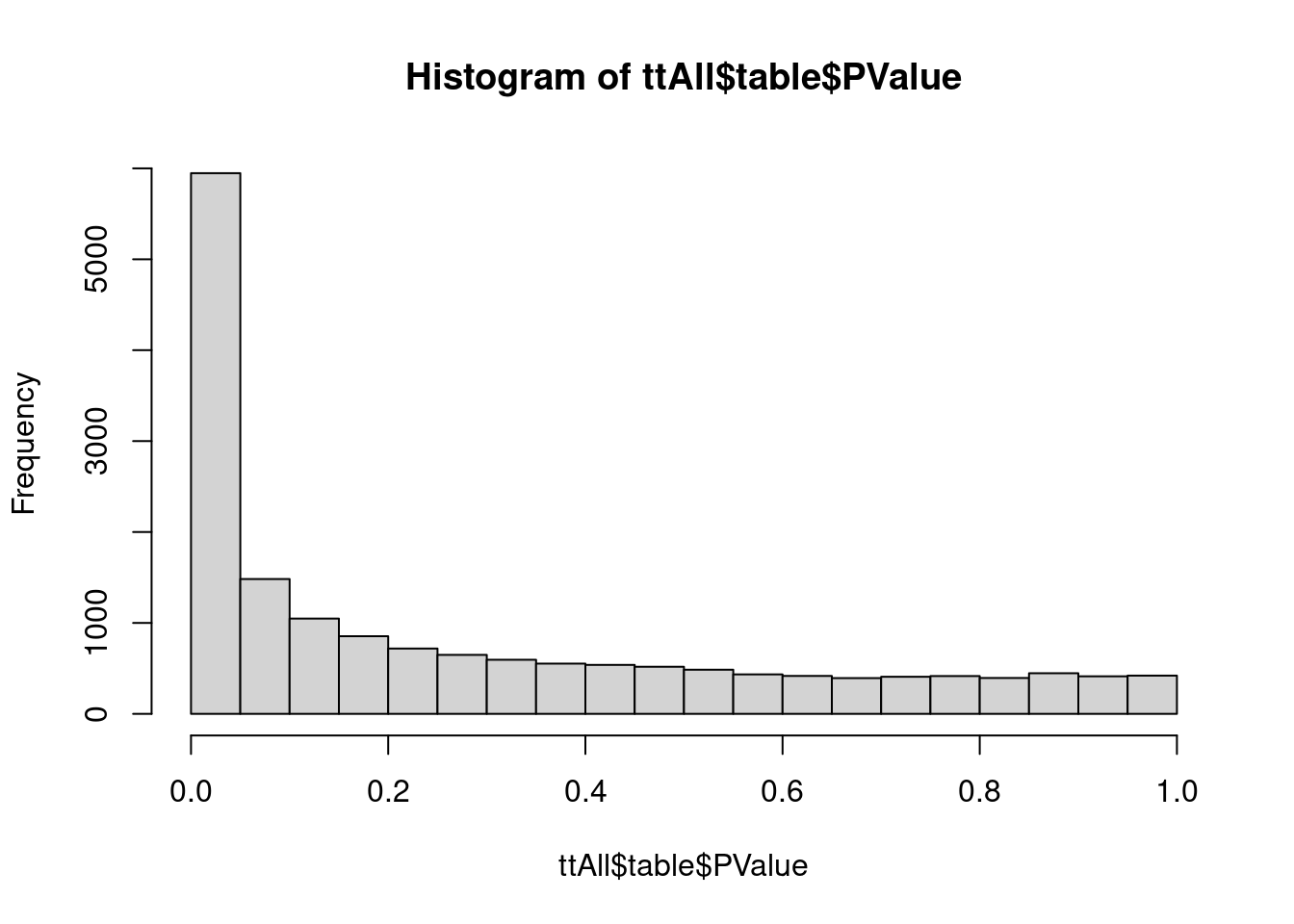

tt <- topTags(ftest, n = nrow(dge), p.value = 0.05) # genes with adj.p<0.05
head(tt)

## Coefficient:  treatmentDexamethasone 
##                               gene_id       tx_ids  SYMBOL     logFC   logCPM
## ENSG00000168309.17 ENSG00000168309.17 ENST0000.... FAM107A  4.735227 2.765893
## ENSG00000109906.13 ENSG00000109906.13 ENST0000....  ZBTB16  6.453612 4.098198
## ENSG00000157214.13 ENSG00000157214.13 ENST0000....  STEAP2  2.017305 7.076725
## ENSG00000162614.18 ENSG00000162614.18 ENST0000....    NEXN  2.028758 7.972003
## ENSG00000120129.5   ENSG00000120129.5 ENST0000....   DUSP1  2.949252 7.262409
## ENSG00000146250.6   ENSG00000146250.6 ENST0000....  PRSS35 -2.728290 3.840471
##                           F       PValue          FDR
## ENSG00000168309.17 697.1081 4.991494e-10 8.552926e-06
## ENSG00000109906.13 895.1711 4.051779e-09 2.463565e-05
## ENSG00000157214.13 814.8833 5.331818e-09 2.463565e-05
## ENSG00000162614.18 735.9130 7.823687e-09 2.463565e-05
## ENSG00000120129.5  688.0311 1.007503e-08 2.463565e-05
## ENSG00000146250.6  667.4199 1.130580e-08 2.463565e-05

nrow(tt)

## [1] 3848

3.6 Plots

We first make a volcanoplot and an MA plot.

library(ggplot2)
volcano <-  ggplot(ttAll$table,aes(x=logFC,y=-log10(PValue),color=FDR<0.05)) + geom_point() + scale_color_manual(values=c("black","red"))
volcano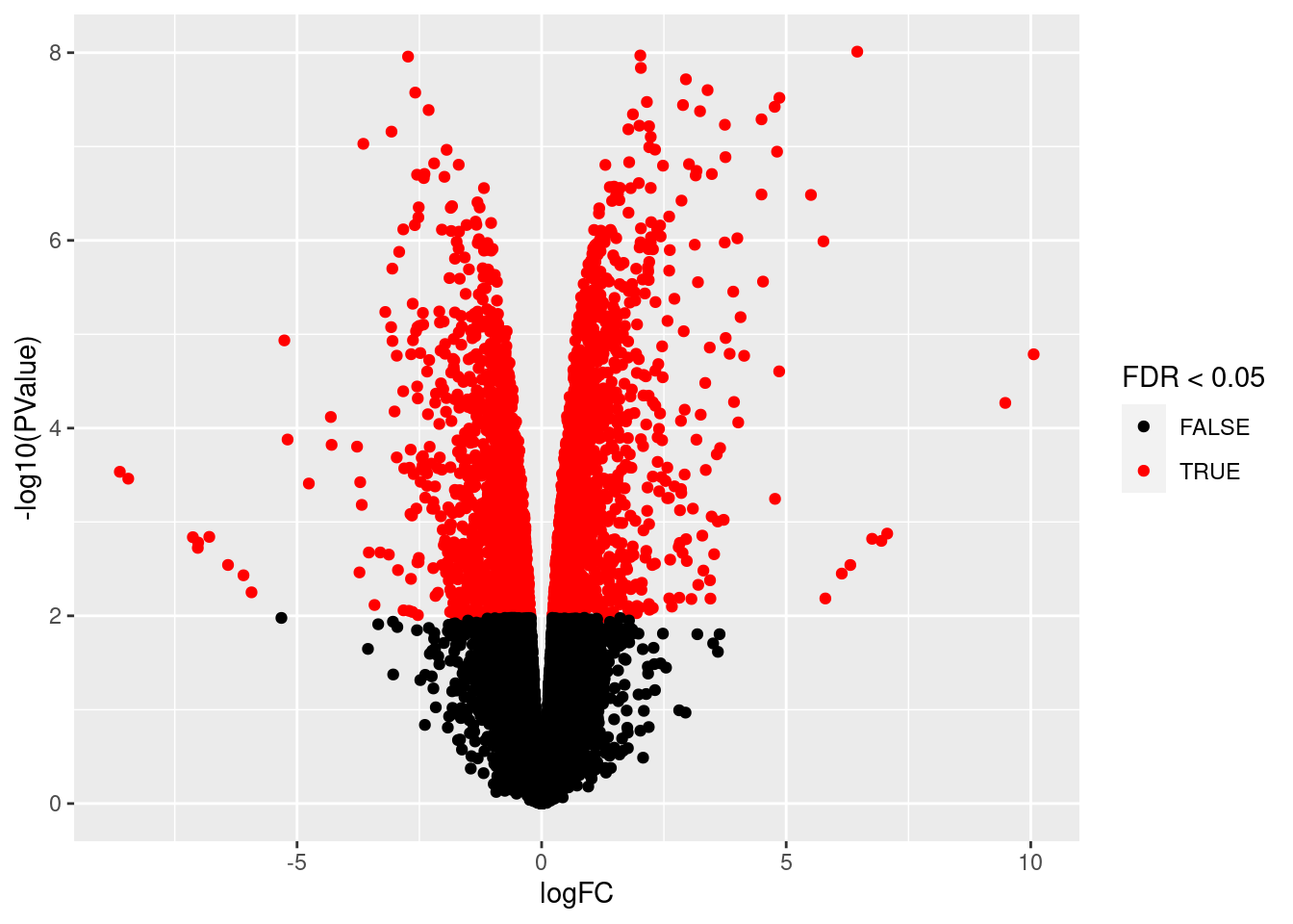

plotSmear(ftest, de.tags = row.names(tt$table))

## Warning in plot.xy(xy.coords(x, y), type = type, ...): "panel.first" is not a
## graphical parameter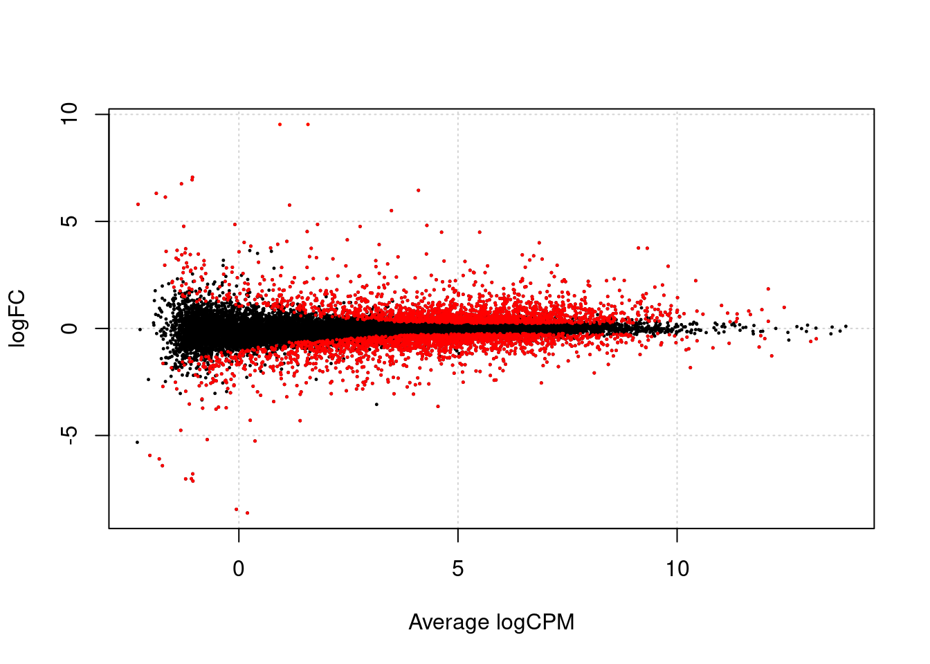

heatmap(cpm(dge,log=TRUE)[rownames(tt$table)[1:30],])

4 Transcript level analysis

4.1 Setup count table

dte <- DGEList(assays(st)$counts)
design <- model.matrix(~treatment+cellLine,data=colData(st))
keep <- filterByExpr(dte, design)
dte <- dte[keep, ,keep.lib.sizes=FALSE]
dte <- calcNormFactors(dte)
dte$samples

4.2 Data Exploration

colnames(dte) <- paste0(substr(pdata$cellLine,1,3),"_",substr(pdata$treatment,1,3))
plotMDS(dte, top = 500,col=as.double(colData(st)$cellLine))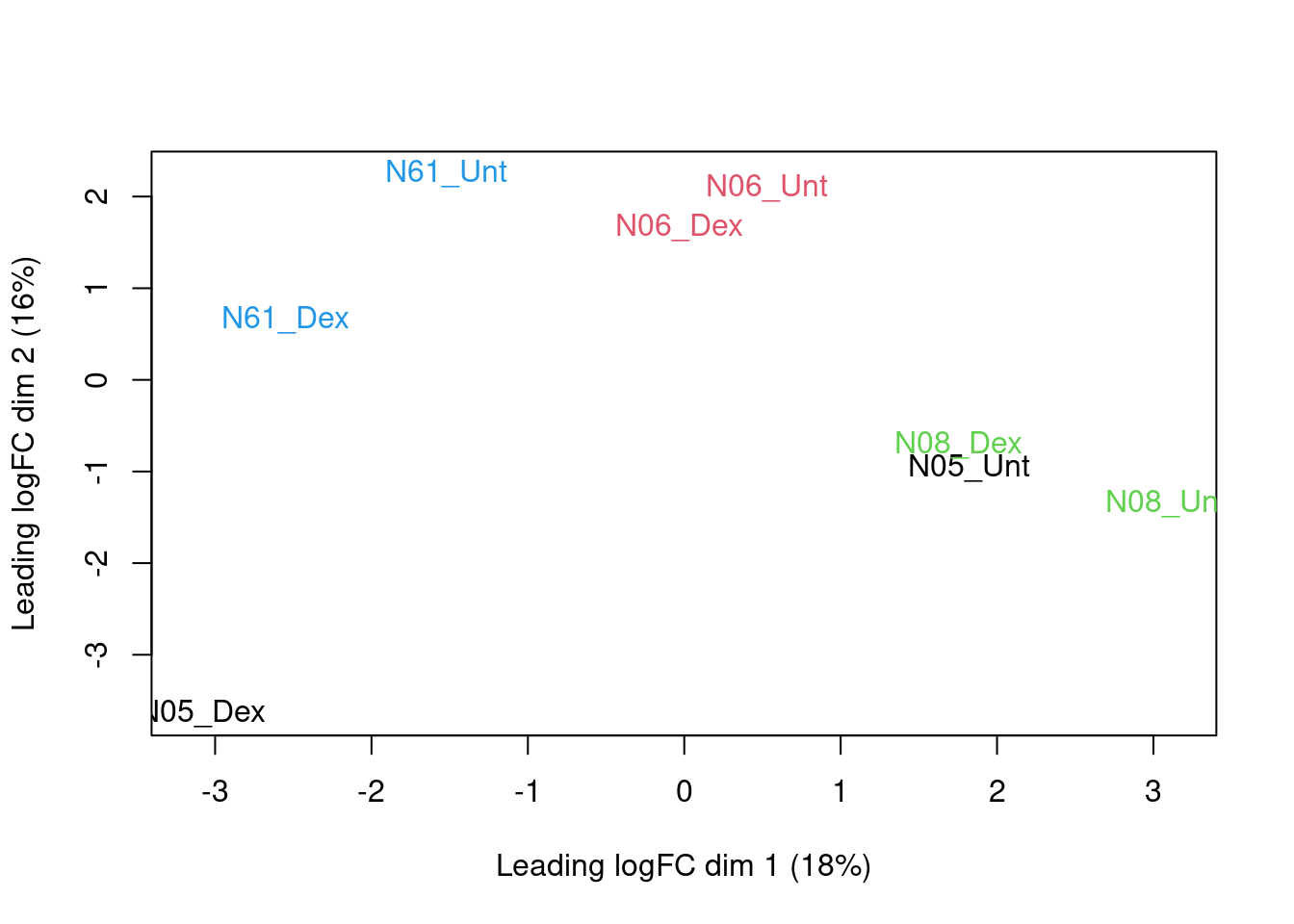

4.3 Model

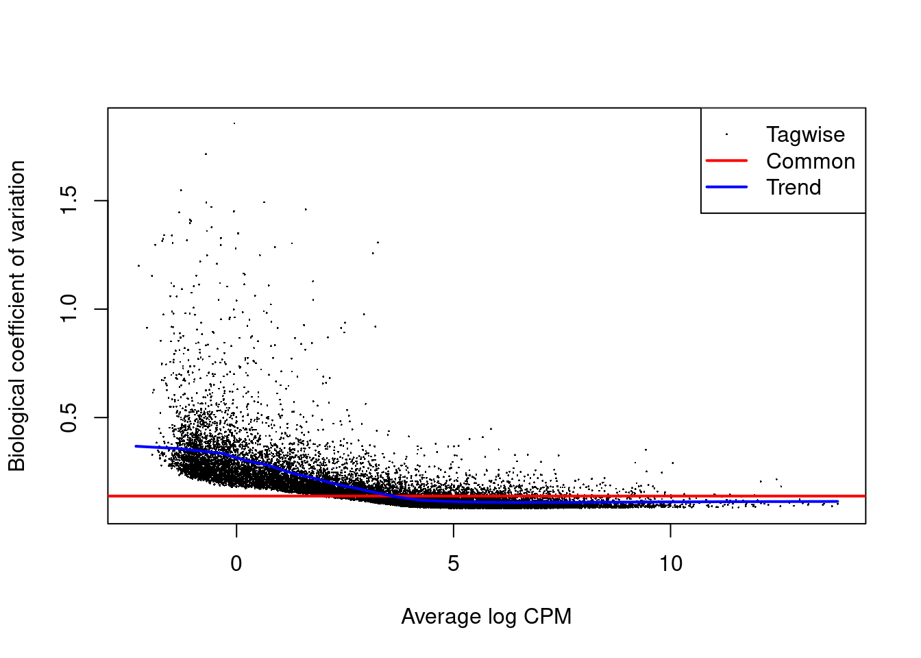
4.3.1 Estimate transcript level dispersion

dte <- estimateDisp(dte, design)
plotBCV(dte)

Note that we observe problems with respect to the dispersion estimation!

This is probably due to over excess zero’s with respect to the NB distribution.

We have seen similar patterns in the counts of plate based single cell RNA-seq data that are not using UMI’s (unique molecular identifiers).

4.3.2 Fit the transcript level quasi-NB model.

fitt <- glmQLFit(dte, design)
ftestt <- glmQLFTest(fitt, coef = "treatmentDexamethasone")
tttAll <- topTags(ftestt, n = nrow(dge)) # all genes
hist(tttAll$table$PValue)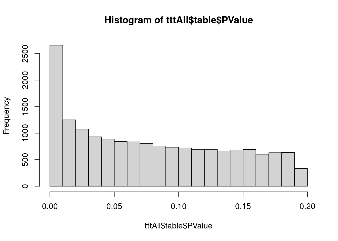

ttt <- topTags(ftestt, n = nrow(dge), p.value = 0.05) # genes with adj.p<0.05
head(ttt)

## Coefficient:  treatmentDexamethasone 
##                        logFC     logCPM        F       PValue          FDR
## ENST00000335953.8   8.525920  4.0739507 435.8649 7.356584e-09 0.0004144479
## ENST00000393080.8   3.306889  4.9144588 951.4920 6.919926e-07 0.0121925655
## ENST00000519214.5   4.155862  0.6574504 148.8974 8.504103e-07 0.0121925655
## ENST00000330010.12  1.884070  7.6321123 866.3483 8.656880e-07 0.0121925655
## ENST00000225964.9  -1.324950 12.1351091 579.1516 2.350564e-06 0.0130232045
## ENST00000429713.6   1.650067  8.5710427 574.7755 2.395151e-06 0.0130232045

nrow(ttt)

## [1] 747

4.4 Plots

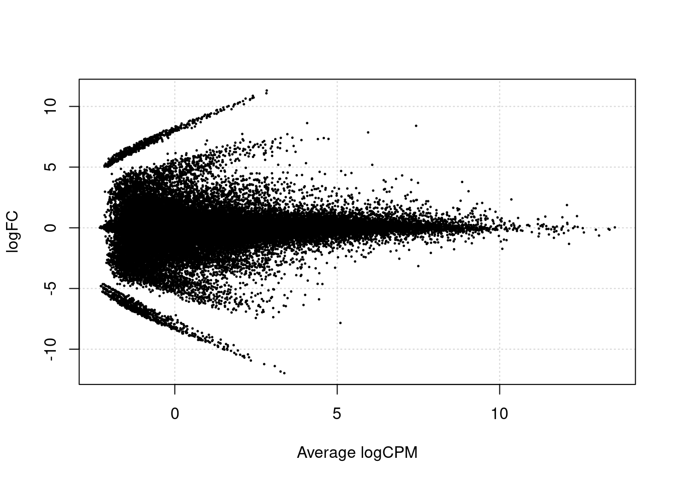
We first make a volcanoplot and an MA plot.

library(ggplot2)
volcano <-  ggplot(tttAll$table,aes(x=logFC,y=-log10(PValue),color=FDR<0.05)) + geom_point() + scale_color_manual(values=c("black","red"))
volcano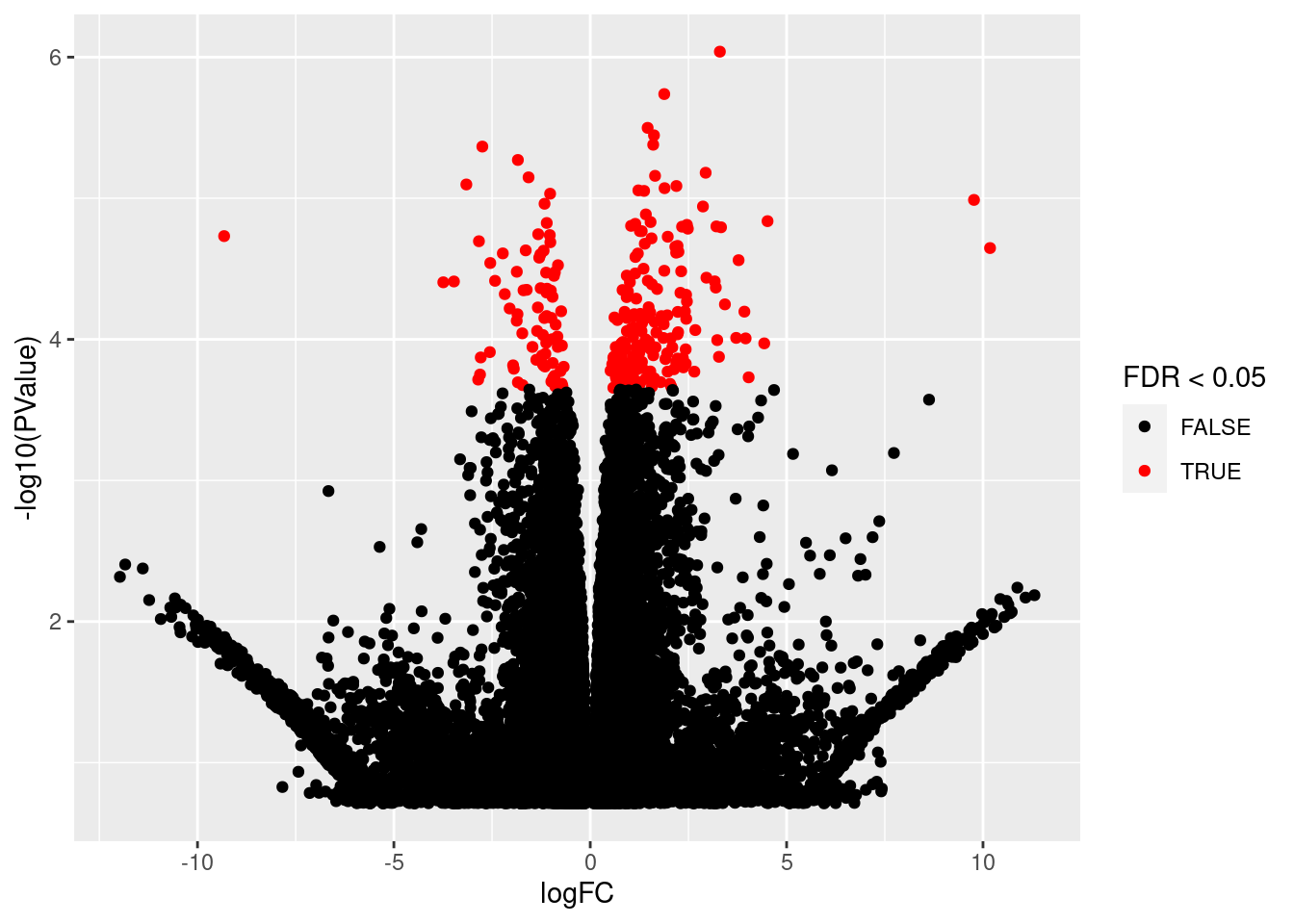

plotSmear(ftestt, de.tags = row.names(tt$table))

## Warning in plot.xy(xy.coords(x, y), type = type, ...): "panel.first" is not a
## graphical parameter

heatmap(cpm(dte,log=TRUE)[rownames(ttt$table)[1:30],])