Experimental design concepts for label-free proteomics experiments

This is part of the online course Experimental Design and Data-Analysis in Label-Free Quantitative LC/MS Proteomics - A Tutorial with msqrob2 (hupo21)

Click to see libraries that are loaded

library(tidyverse)
library(limma)
library(QFeatures)
library(msqrob2)
library(plotly)
library(gridExtra)

1 Overview

• Sample size
• Randomized Complete Block Designs

2 Sample size

2.1 Statistical models

• Upon preprocessing and summarization we model the log2 transformed protein expression (\(y_{i}\)) values using a linear model

\[y_{i}= \beta_0 + \beta_1 x_{i,1} + \beta x_{i,2} + ... + \epsilon_i\]

with

• \(\beta_0\) the intercept
• \(\beta_j\) the slope for predictor \(x_{i,j}\)
• \(x_{i,j}\) a continuous predictor (such as age) or a dummy variable that can take values of 0 and 1 and that will used for factors (e.g treatment: cancer, normal).

Example:

• Estrogen Receptor Positive Breast cancer tissues from from patients treated with tamoxifen upon recurrence have been assessed in a proteomics study.
• Half of the patients had a good outcome (or) and the other half had a poor outcome (pd).
• The proteomes have been assessed using an LTQ-Orbitrap and the thermo output .RAW files were searched with MaxQuant (version 1.4.1.2) against the human proteome database (FASTA version 2012-09, human canonical proteome).

We model the data for a single protein using a model:

\[y_{i}= \beta_0 + \beta_{PD} x_{i,PD} + \epsilon_i\]

with \(x_{i,PD}=\begin{cases} 0& \text{good outcome}\\ 1& \text{poor outcome} \end{cases}\).

2.1.1 Read data

Click to see background and code

1. We use a peptides.txt file from MS-data quantified with maxquant that contains MS1 intensities summarized at the peptide level.

peptidesFile <- "https://raw.githubusercontent.com/statOmics/pda21/data/quantification/cancer/peptides3vs3.txt"

2. Maxquant stores the intensity data for the different samples in columnns that start with Intensity. We can retreive the column names with the intensity data with the code below:

ecols <- grep("Intensity\\.", names(read.delim(peptidesFile)))

3. Read the data and store it in QFeatures object

pe <- readQFeatures(
  table = peptidesFile,
  fnames = 1,
  ecol = ecols,
  name = "peptideRaw", sep="\t")

2.1.2 Design

Click to see background and code

pe %>% colnames

## CharacterList of length 1
## [["peptideRaw"]] Intensity.OR.01 Intensity.OR.04 ... Intensity.PD.04

• Note, that the sample names the outcome.
• We update the colData with information on the design

colData(pe)$prognosis <-  pe[["peptideRaw"]] %>% 
  colnames %>% 
  substr(11,12) %>% 
  as.factor

• We explore the colData

colData(pe)

## DataFrame with 6 rows and 1 column
##                 prognosis
##                  <factor>
## Intensity.OR.01        OR
## Intensity.OR.04        OR
## Intensity.OR.07        OR
## Intensity.PD.02        PD
## Intensity.PD.03        PD
## Intensity.PD.04        PD

2.1.3 Preprocessing

Click to see code for preprocessing

1. Log-transform

• We calculate how many non zero intensities we have for each peptide and this can be useful for filtering.

rowData(pe[["peptideRaw"]])$nNonZero <- rowSums(assay(pe[["peptideRaw"]]) > 0)

• Peptides with zero intensities are missing peptides and should be represent with a NA value rather than 0.

pe <- zeroIsNA(pe, "peptideRaw") # convert 0 to NA

• Logtransform data with base 2

pe <- logTransform(pe, base = 2, i = "peptideRaw", name = "peptideLog")

2. Filtering

Click to see code to filter the data

• Handling overlapping protein groups

In our approach a peptide can map to multiple proteins, as long as there is none of these proteins present in a smaller subgroup.

pe <- filterFeatures(pe, ~ Proteins %in% smallestUniqueGroups(rowData(pe[["peptideLog"]])$Proteins))

• Remove reverse sequences (decoys) and contaminants

We now remove the contaminants, peptides that map to decoy sequences, and proteins which were only identified by peptides with modifications.

pe <- filterFeatures(pe,~Reverse != "+")
pe <- filterFeatures(pe,~ Contaminant != "+")

• Drop peptides that were only identified in one sample

We keep peptides that were observed at last twice.

pe <- filterFeatures(pe,~ nNonZero >=2)
nrow(pe[["peptideLog"]])

## [1] 22413

We keep 22413 peptides upon filtering.

3. Normalization

pe <- normalize(pe, 
                i = "peptideLog", 
                name = "peptideNorm", 
                method = "center.median")

4. Summarization

pe <- aggregateFeatures(pe,
  i = "peptideNorm",
  fcol = "Proteins",
  na.rm = TRUE,
  name = "protein")

2.2 Effect size?

library(ExploreModelMatrix)
VisualizeDesign(colData(pe),designFormula = ~prognosis)$plotlist

## [[1]]

\[ \begin{array}{rclcl} E[Y|OR] &=& \beta_0\\ E[Y|PD] &=& \beta_0 + \beta_{PD}\\ \log_2 FC_{PD-OR} &=& \beta_0 + \beta_{PD} - \beta_0 &=&\beta_{PD} \end{array} \]

2.3 Statistical Inference

2.3.1 Hypotheses

We want to find proteins that are differential abundant

\(\rightarrow\) use a statistical test

We typically start from the alternative hypothesis

• \(H_1\): \(\log_2 FC_{PD-OR} \neq 0\) or \(\beta_{PD} \neq 0\)

But we can not use data to prove a hypothesis, we therefore falsify the opposite:

• \(H_0\): \(\log_2 FC_{PD-OR} = 0\) or \(\beta_{PD} = 0\)

2.3.2 Test statistic:

• T-test on the model parameter \(\beta_{PD}\)

\[T = \frac{\hat\beta_{PD} - 0}{\text{se}_{\hat\beta_{PD}}}\]

which follows a t-distribution under \(H_0\) if the errors are \[ \epsilon_i \text{ i.i.d. } N(0,\sigma^2) \]

• p-value: probability to observe a t-statistic that is as extreme or more extreme that the one we observed for this protein in our sample if we would repeat the experiment and if the protein is not differentially abundant.

2.3.3 Multiple testing

• We do this test for all proteins (typically thousands of them)

• Adjust p-values for multiple testing using the false discovery rate \[FDR = E\left[\frac{FP}{FP + TP}\right]\]

• Empirical Bayes variance estimation: Note, that the massive parallel data structure also allows you to stabilize the variance estimation by borrowing information across proteins!

Note, if you want to refresh some fundamental concepts of hypothesis testing:

• Statistical hypothesis testing
• Multiple hypothesis testing
• Empirical Bayes Variance Estimation

2.4 Experiment with 3 vs 3 comparison

Click to see code to inference

pe <- msqrob(object = pe, i = "protein", formula = ~prognosis)
L <- makeContrast("prognosisPD=0", parameterNames = c("prognosisPD"))
pe <- hypothesisTest(object = pe, i = "protein", contrast = L)

volcano3x3 <- ggplot(rowData(pe[["protein"]])$prognosisPD %>% na.exclude,
                  aes(x = logFC, y = -log10(pval), color = adjPval < 0.05)) +
  geom_point(cex = 2.5) +
  scale_color_manual(values = alpha(c("black", "red"), 0.5)) + 
  theme_minimal() +
  ggtitle(paste0(sum(rowData(pe[["protein"]])$prognosisPD$adjPval<0.05,na.rm=TRUE)," proteins are found to be DA"))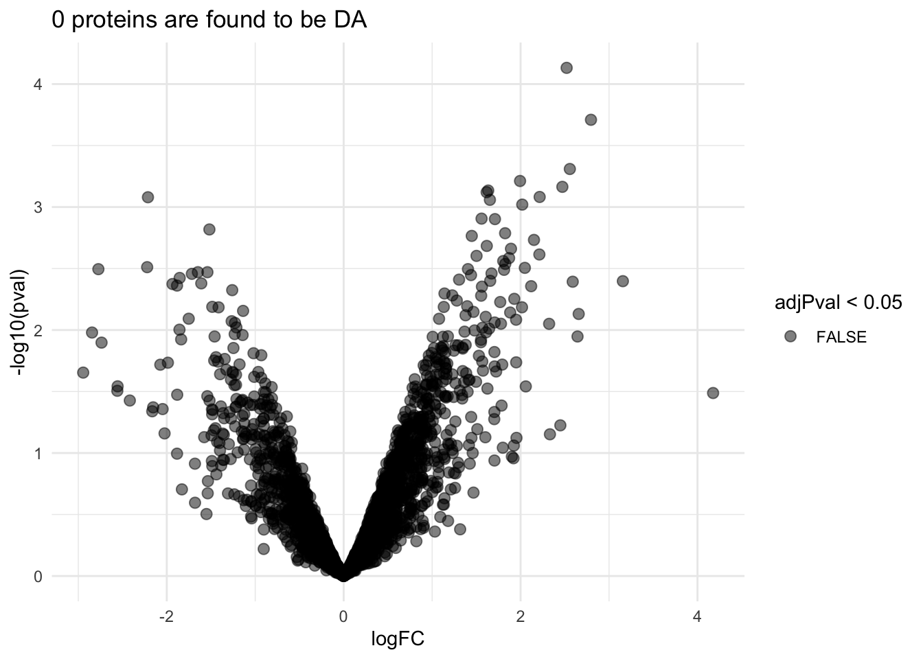

volcano3x3

Upon correction for multiple testing with using the false discovery rate (FDR) method no proteins are found to be differentially expressed.

Note, that you can refresh the concept of multiple testing and FDR [here] (https://statomics.github.io/PDA21/pda_quantification_inference.html#14_Multiple_hypothesis_testing).

2.5 Experiment with a 6 vs 6 comparison

2.5.1 Read data

Click to see background and code

1. We use a peptides.txt file from MS-data quantified with maxquant that contains MS1 intensities summarized at the peptide level.

peptidesFile <- "https://raw.githubusercontent.com/statOmics/pda21/data/quantification/cancer/peptides6vs6.txt"

2. Maxquant stores the intensity data for the different samples in columnns that start with Intensity. We can retreive the column names with the intensity data with the code below:

ecols <- grep("Intensity\\.", names(read.delim(peptidesFile)))

3. Read the data and store it in QFeatures object

pe <- readQFeatures(
  table = peptidesFile,
  fnames = 1,
  ecol = ecols,
  name = "peptideRaw", sep="\t")

2.5.2 Design

Click to see background and code

pe %>% colnames

## CharacterList of length 1
## [["peptideRaw"]] Intensity.OR.01 Intensity.OR.04 ... Intensity.PD.08

• Note, that the sample names the outcome.
• We update the colData with information on the design

colData(pe)$prognosis <-  pe[["peptideRaw"]] %>% 
  colnames %>% 
  substr(11,12) %>% 
  as.factor

• We explore the colData

colData(pe)

## DataFrame with 12 rows and 1 column
##                 prognosis
##                  <factor>
## Intensity.OR.01        OR
## Intensity.OR.04        OR
## Intensity.OR.07        OR
## Intensity.OR.09        OR
## Intensity.OR.10        OR
## ...                   ...
## Intensity.PD.03        PD
## Intensity.PD.04        PD
## Intensity.PD.06        PD
## Intensity.PD.07        PD
## Intensity.PD.08        PD

2.5.3 Preprocessing

Click to see code for preprocessing

1. Log-transform

• We calculate how many non zero intensities we have for each peptide and this can be useful for filtering.

rowData(pe[["peptideRaw"]])$nNonZero <- rowSums(assay(pe[["peptideRaw"]]) > 0)

• Peptides with zero intensities are missing peptides and should be represent with a NA value rather than 0.

pe <- zeroIsNA(pe, "peptideRaw") # convert 0 to NA

• Logtransform data with base 2

pe <- logTransform(pe, base = 2, i = "peptideRaw", name = "peptideLog")

2. Filtering

Click to see code to filter the data

• Handling overlapping protein groups

In our approach a peptide can map to multiple proteins, as long as there is none of these proteins present in a smaller subgroup.

pe <- filterFeatures(pe, ~ Proteins %in% smallestUniqueGroups(rowData(pe[["peptideLog"]])$Proteins))

• Remove reverse sequences (decoys) and contaminants

We now remove the contaminants, peptides that map to decoy sequences, and proteins which were only identified by peptides with modifications.

pe <- filterFeatures(pe,~Reverse != "+")
pe <- filterFeatures(pe,~ Contaminant != "+")

• Drop peptides that were only identified in one sample

We keep peptides that were observed at last twice.

pe <- filterFeatures(pe,~ nNonZero >=2)
nrow(pe[["peptideLog"]])

## [1] 25452

We keep 25452 peptides upon filtering.

3. Normalization

pe <- normalize(pe, 
                i = "peptideLog", 
                name = "peptideNorm", 
                method = "center.median")

4. Summarization

pe <- aggregateFeatures(pe,
  i = "peptideNorm",
  fcol = "Proteins",
  na.rm = TRUE,
  name = "protein")

2.5.4 Statistical Inference

Click to see code to inference

pe <- msqrob(object = pe, i = "protein", formula = ~prognosis)
L <- makeContrast("prognosisPD=0", parameterNames = c("prognosisPD"))
pe <- hypothesisTest(object = pe, i = "protein", contrast = L)

volcano6x6 <- ggplot(rowData(pe[["protein"]])$prognosisPD %>% na.exclude,
                  aes(x = logFC, y = -log10(pval), color = adjPval < 0.05)) +
  geom_point(cex = 2.5) +
  scale_color_manual(values = alpha(c("black", "red"), 0.5)) + 
  theme_minimal() +
  ggtitle(paste0(sum(rowData(pe[["protein"]])$prognosisPD$adjPval<0.05,na.rm=TRUE)," proteins are found to be DA"))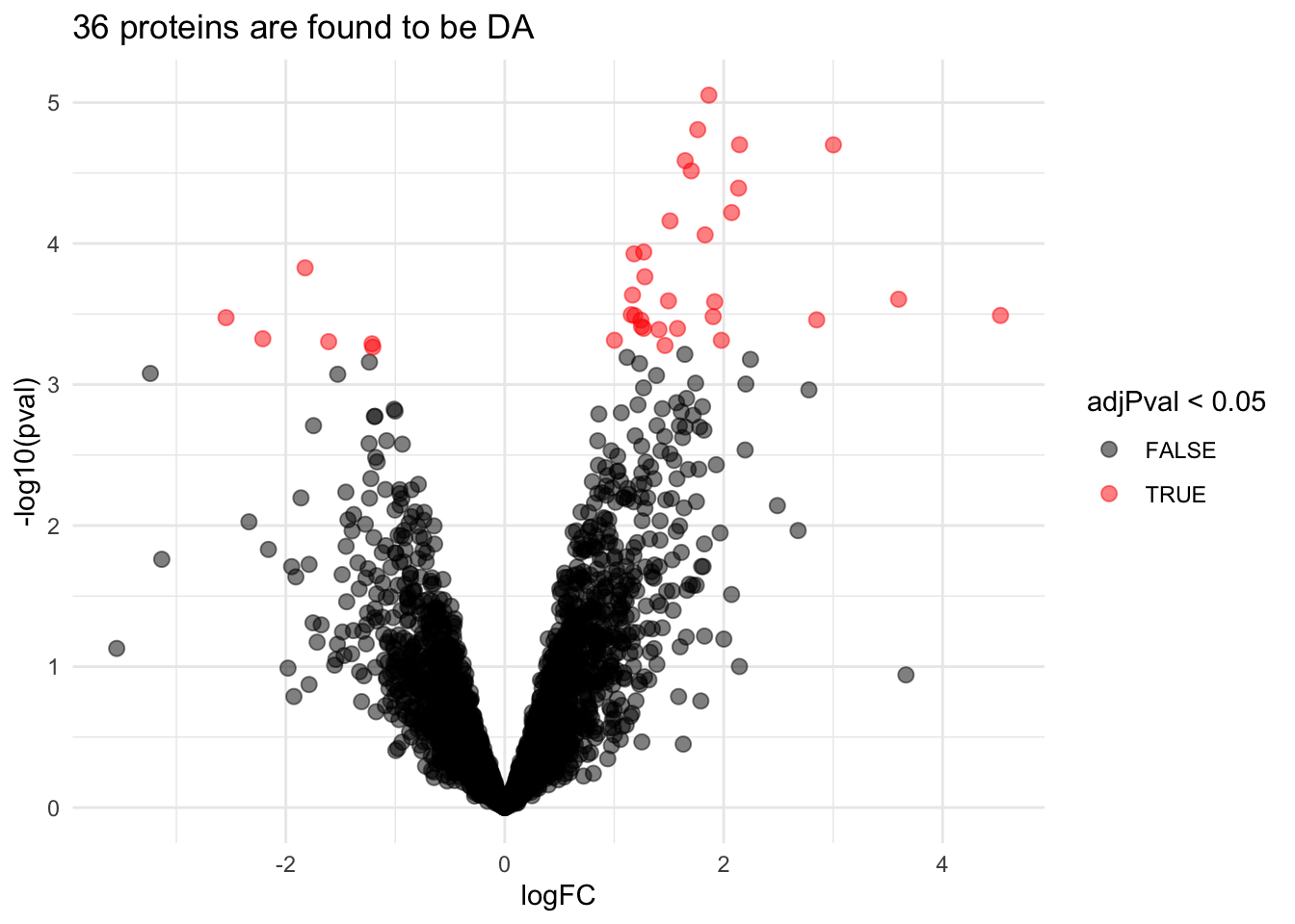

volcano6x6

2.6 Experiment with a 9 vs 9 comparison

2.6.1 Read data

Click to see background and code

1. We use a peptides.txt file from MS-data quantified with maxquant that contains MS1 intensities summarized at the peptide level.

peptidesFile <- "https://raw.githubusercontent.com/statOmics/pda21/data/quantification/cancer/peptides9vs9.txt"

2. Maxquant stores the intensity data for the different samples in columnns that start with Intensity. We can retreive the column names with the intensity data with the code below:

ecols <- grep("Intensity\\.", names(read.delim(peptidesFile)))

3. Read the data and store it in QFeatures object

pe <- readQFeatures(
  table = peptidesFile,
  fnames = 1,
  ecol = ecols,
  name = "peptideRaw", sep="\t")

2.6.2 Design

Click to see background and code

pe %>% colnames

## CharacterList of length 1
## [["peptideRaw"]] Intensity.OR.01 Intensity.OR.04 ... Intensity.PD.11

• Note, that the sample names the outcome.
• We update the colData with information on the design

colData(pe)$prognosis <-  pe[["peptideRaw"]] %>% 
  colnames %>% 
  substr(11,12) %>% 
  as.factor

• We explore the colData

colData(pe)

## DataFrame with 18 rows and 1 column
##                 prognosis
##                  <factor>
## Intensity.OR.01        OR
## Intensity.OR.04        OR
## Intensity.OR.07        OR
## Intensity.OR.09        OR
## Intensity.OR.10        OR
## ...                   ...
## Intensity.PD.07        PD
## Intensity.PD.08        PD
## Intensity.PD.09        PD
## Intensity.PD.10        PD
## Intensity.PD.11        PD

2.6.3 Preprocessing

Click to see code for preprocessing

1. Log-transform

• We calculate how many non zero intensities we have for each peptide and this can be useful for filtering.

rowData(pe[["peptideRaw"]])$nNonZero <- rowSums(assay(pe[["peptideRaw"]]) > 0)

• Peptides with zero intensities are missing peptides and should be represent with a NA value rather than 0.

pe <- zeroIsNA(pe, "peptideRaw") # convert 0 to NA

• Logtransform data with base 2

pe <- logTransform(pe, base = 2, i = "peptideRaw", name = "peptideLog")

2. Filtering

Click to see code to filter the data

• Handling overlapping protein groups

In our approach a peptide can map to multiple proteins, as long as there is none of these proteins present in a smaller subgroup.

pe <- filterFeatures(pe, ~ Proteins %in% smallestUniqueGroups(rowData(pe[["peptideLog"]])$Proteins))

• Remove reverse sequences (decoys) and contaminants

We now remove the contaminants, peptides that map to decoy sequences, and proteins which were only identified by peptides with modifications.

pe <- filterFeatures(pe,~Reverse != "+")
pe <- filterFeatures(pe,~ Contaminant != "+")

• Drop peptides that were only identified in one sample

We keep peptides that were observed at last twice.

pe <- filterFeatures(pe,~ nNonZero >=2)
nrow(pe[["peptideLog"]])

## [1] 26696

We keep 26696 peptides upon filtering.

3. Normalization

pe <- normalize(pe, 
                i = "peptideLog", 
                name = "peptideNorm", 
                method = "center.median")

4. Summarization

pe <- aggregateFeatures(pe,
  i = "peptideNorm",
  fcol = "Proteins",
  na.rm = TRUE,
  name = "protein")

2.6.4 Statistical Inference

Click to see code to inference

pe <- msqrob(object = pe, i = "protein", formula = ~prognosis)
L <- makeContrast("prognosisPD=0", parameterNames = c("prognosisPD"))
pe <- hypothesisTest(object = pe, i = "protein", contrast = L)

volcano9x9 <- ggplot(rowData(pe[["protein"]])$prognosisPD %>% na.exclude,
                  aes(x = logFC, y = -log10(pval), color = adjPval < 0.05)) +
  geom_point(cex = 2.5) +
  scale_color_manual(values = alpha(c("black", "red"), 0.5)) + 
  theme_minimal() +
  ggtitle(paste0(sum(rowData(pe[["protein"]])$prognosisPD$adjPval<0.05,na.rm=TRUE)," proteins are found to be DA"))

volcano9x9

• We have seen that the sample size is key to recover DA proteins

• Indeed, if a protein is differentially expressed, the value of T-test depends on the effect size, the variability of the protein expression values and the sample size.

\[ T_g=\frac{\log_2 \text{FC}}{\text{se}_{\log_2 \text{FC}}} \]

\[ T_g=\frac{\widehat{\text{signal}}}{\widehat{\text{Noise}}} \]

For a two group comparison the standard error on the fold change equals

\[ \text{se}_{\log_2 \text{FC}}=\text{SD}\sqrt{\frac{1}{n_1}+\frac{1}{n_2}} \]

\(\rightarrow\) if number of bio-repeats increases we have a higher power!

3 Randomized complete block designs

\[\sigma^2= \sigma^2_{bio}+\sigma^2_\text{lab} +\sigma^2_\text{extraction} + \sigma^2_\text{run} + \ldots\]

• Biological: fluctuations in protein level between mice, fluctations in protein level between cells, …
• Technical: cage effect, lab effect, week effect, plasma extraction, MS-run, …

3.1 Nature methods: Points of significance - Blocking

https://www.nature.com/articles/nmeth.3005.pdf

3.2 Mouse example

Duguet et al. (2017) MCP 16(8):1416-1432. doi: 10.1074/mcp.m116.062745

• All treatments of interest are present within block!
• We can estimate the effect of the treatment within block!

To illustrate the power of blocking we have subsetted the data of Duguet et al. in a

• completely randomized design with

  • four mice for which we only have measurements on the ordinary T-cells
  • four mice for which we only have measurements on the regulatory T-cells

• randomized complete block design with four mice for which we both have

  • measurements on ordinary T-cells as well as
  • measurements on regulatory T-cells

3.2.1 Data

Click to see code

library(tidyverse)
library(limma)
library(QFeatures)
library(msqrob2)
library(plotly)
library(gridExtra)

peptidesFile <- "https://raw.githubusercontent.com/statOmics/PDA21/data/quantification/mouseTcell/peptidesRCB.txt"
peptidesFile2 <- "https://raw.githubusercontent.com/statOmics/PDA21/data/quantification/mouseTcell/peptidesCRD.txt"
peptidesFile3 <- "https://raw.githubusercontent.com/statOmics/PDA21/data/quantification/mouseTcell/peptides.txt"

ecols <- grep("Intensity\\.", names(read.delim(peptidesFile)))
pe <- readQFeatures(
  table = peptidesFile,
  fnames = 1,
  ecol = ecols,
  name = "peptideRaw", sep="\t")

ecols2 <- grep("Intensity\\.", names(read.delim(peptidesFile2)))
pe2 <- readQFeatures(
  table = peptidesFile2,
  fnames = 1,
  ecol = ecols2,
  name = "peptideRaw", sep="\t")

ecols3 <- grep("Intensity\\.", names(read.delim(peptidesFile3)))
pe3 <- readQFeatures(
  table = peptidesFile3,
  fnames = 1,
  ecol = ecols3,
  name = "peptideRaw", sep="\t")

### Design
colData(pe)$celltype <- substr(
  colnames(pe[["peptideRaw"]]),
  11,
  14) %>%
  unlist %>%  
  as.factor

colData(pe)$mouse <- pe[[1]] %>%
  colnames %>%
  strsplit(split="[.]")  %>%
  sapply(function(x) x[3]) %>%
  as.factor

colData(pe2)$celltype <- substr(
  colnames(pe2[["peptideRaw"]]),
  11,
  14) %>%
  unlist %>%  
  as.factor

colData(pe2)$mouse <- pe2[[1]] %>%
  colnames %>%
  strsplit(split="[.]")  %>%
  sapply(function(x) x[3]) %>%
  as.factor

colData(pe3)$celltype <- substr(
  colnames(pe3[["peptideRaw"]]),
  11,
  14) %>%
  unlist %>%  
  as.factor

colData(pe3)$mouse <- pe3[[1]] %>%
  colnames %>%
  strsplit(split="[.]")  %>%
  sapply(function(x) x[3]) %>%
  as.factor

3.2.2 Preprocessing

3.2.2.1 Log-transform

Click to see code to log-transfrom the data

• We calculate how many non zero intensities we have for each peptide and this can be useful for filtering.

rowData(pe[["peptideRaw"]])$nNonZero <- rowSums(assay(pe[["peptideRaw"]]) > 0)

rowData(pe2[["peptideRaw"]])$nNonZero <- rowSums(assay(pe2[["peptideRaw"]]) > 0)

rowData(pe3[["peptideRaw"]])$nNonZero <- rowSums(assay(pe3[["peptideRaw"]]) > 0)

• Peptides with zero intensities are missing peptides and should be represent with a NA value rather than 0.

pe <- zeroIsNA(pe, "peptideRaw") # convert 0 to NA

pe2 <- zeroIsNA(pe2, "peptideRaw") # convert 0 to NA

pe3 <- zeroIsNA(pe3, "peptideRaw") # convert 0 to NA

• Logtransform data with base 2

pe <- logTransform(pe, base = 2, i = "peptideRaw", name = "peptideLog")

pe2 <- logTransform(pe2, base = 2, i = "peptideRaw", name = "peptideLog")

pe3 <- logTransform(pe3, base = 2, i = "peptideRaw", name = "peptideLog")

3.2.2.2 Filtering

Click to see details on filtering

1. Handling overlapping protein groups

In our approach a peptide can map to multiple proteins, as long as there is none of these proteins present in a smaller subgroup.

pe <- filterFeatures(pe, ~ Proteins %in% smallestUniqueGroups(rowData(pe[["peptideLog"]])$Proteins))

pe2 <- filterFeatures(pe2, ~ Proteins %in% smallestUniqueGroups(rowData(pe2[["peptideLog"]])$Proteins))

pe3 <- filterFeatures(pe3, ~ Proteins %in% smallestUniqueGroups(rowData(pe3[["peptideLog"]])$Proteins))

2. Remove reverse sequences (decoys) and contaminants

We now remove the contaminants, peptides that map to decoy sequences, and proteins which were only identified by peptides with modifications.

pe <- filterFeatures(pe,~Reverse != "+")
pe <- filterFeatures(pe,~ Potential.contaminant != "+")

pe2 <- filterFeatures(pe2,~Reverse != "+")
pe2 <- filterFeatures(pe2,~ Potential.contaminant != "+")

pe3 <- filterFeatures(pe3,~Reverse != "+")
pe3 <- filterFeatures(pe3,~ Potential.contaminant != "+")

3. Drop peptides that were only identified in one sample

We keep peptides that were observed at last twice.

pe <- filterFeatures(pe,~ nNonZero >=2)
nrow(pe[["peptideLog"]])

## [1] 44449

pe2 <- filterFeatures(pe2,~ nNonZero >=2)
nrow(pe2[["peptideLog"]])

## [1] 43401

pe3 <- filterFeatures(pe3,~ nNonZero >=2)
nrow(pe3[["peptideLog"]])

## [1] 47431

3.2.2.3 Normalization

Click to see code to normalize the data

pe <- normalize(pe, 
                i = "peptideLog", 
                name = "peptideNorm", 
                method = "center.median")

pe2 <- normalize(pe2, 
                i = "peptideLog", 
                name = "peptideNorm", 
                method = "center.median")


pe3 <- normalize(pe3, 
                i = "peptideLog", 
                name = "peptideNorm", 
                method = "center.median")

3.2.2.4 Summarization

Click to see code to summarize the data

pe <- aggregateFeatures(pe,
 i = "peptideNorm",
 fcol = "Proteins",
 na.rm = TRUE,
 name = "protein")

## Your quantitative and row data contain missing values. Please read the
## relevant section(s) in the aggregateFeatures manual page regarding the
## effects of missing values on data aggregation.

pe2 <- aggregateFeatures(pe2,
 i = "peptideNorm",
 fcol = "Proteins",
 na.rm = TRUE,
 name = "protein")

## Your quantitative and row data contain missing values. Please read the
## relevant section(s) in the aggregateFeatures manual page regarding the
## effects of missing values on data aggregation.

pe3 <- aggregateFeatures(pe3,
 i = "peptideNorm",
 fcol = "Proteins",
 na.rm = TRUE,
 name = "protein")

## Your quantitative and row data contain missing values. Please read the
## relevant section(s) in the aggregateFeatures manual page regarding the
## effects of missing values on data aggregation.

3.2.3 Data Exploration: what is impact of blocking?

Click to see code

levels(colData(pe3)$mouse) <- paste0("m",1:7)
mdsObj3 <- plotMDS(assay(pe3[["protein"]]), plot = FALSE)
mdsOrig <- colData(pe3) %>%
  as.data.frame %>%
  mutate(mds1 = mdsObj3$x,
         mds2 = mdsObj3$y,
         lab = paste(mouse,celltype,sep="_")) %>%
  ggplot(aes(x = mds1, y = mds2, label = lab, color = celltype, group = mouse)) +
  geom_text(show.legend = FALSE) +
  geom_point(shape = 21) +
  geom_line(color = "black", linetype = "dashed") +
  xlab(
    paste0(
      mdsObj3$axislabel,
      " ",
      1, 
      " (",
      paste0(
        round(mdsObj3$var.explained[1] *100,0),
        "%"
        ),
      ")"
      )
    ) +
  ylab(
    paste0(
      mdsObj3$axislabel,
      " ",
      2, 
      " (",
      paste0(
        round(mdsObj3$var.explained[2] *100,0),
        "%"
        ),
      ")"
      )
    ) +
  ggtitle("Original (RCB)")

levels(colData(pe)$mouse) <- paste0("m",1:4)
mdsObj <- plotMDS(assay(pe[["protein"]]), plot = FALSE)
mdsRCB <- colData(pe) %>%
  as.data.frame %>%
  mutate(mds1 = mdsObj$x,
         mds2 = mdsObj$y,
         lab = paste(mouse,celltype,sep="_")) %>%
  ggplot(aes(x = mds1, y = mds2, label = lab, color = celltype, group = mouse)) +
  geom_text(show.legend = FALSE) +
  geom_point(shape = 21) +
  geom_line(color = "black", linetype = "dashed") +
  xlab(
    paste0(
      mdsObj$axislabel,
      " ",
      1, 
      " (",
      paste0(
        round(mdsObj$var.explained[1] *100,0),
        "%"
        ),
      ")"
      )
    ) +
  ylab(
    paste0(
      mdsObj$axislabel,
      " ",
      2, 
      " (",
      paste0(
        round(mdsObj$var.explained[2] *100,0),
        "%"
        ),
      ")"
      )
    ) +
  ggtitle("Randomized Complete Block (RCB)")


levels(colData(pe2)$mouse) <- paste0("m",1:8)
mdsObj2 <- plotMDS(assay(pe2[["protein"]]), plot = FALSE)
mdsCRD <- colData(pe2) %>%
  as.data.frame %>%
  mutate(mds1 = mdsObj2$x,
         mds2 = mdsObj2$y,
         lab = paste(mouse,celltype,sep="_")) %>%
  ggplot(aes(x = mds1, y = mds2, label = lab, color = celltype, group = mouse)) +
  geom_text(show.legend = FALSE) +
  geom_point(shape = 21) +
  xlab(
    paste0(
      mdsObj$axislabel,
      " ",
      1, 
      " (",
      paste0(
        round(mdsObj2$var.explained[1] *100,0),
        "%"
        ),
      ")"
      )
    ) +
  ylab(
    paste0(
      mdsObj$axislabel,
      " ",
      2, 
      " (",
      paste0(
        round(mdsObj2$var.explained[2] *100,0),
        "%"
        ),
      ")"
      )
    ) +
  ggtitle("Completely Randomized Design (CRD)")

mdsOrig

mdsRCB

mdsCRD

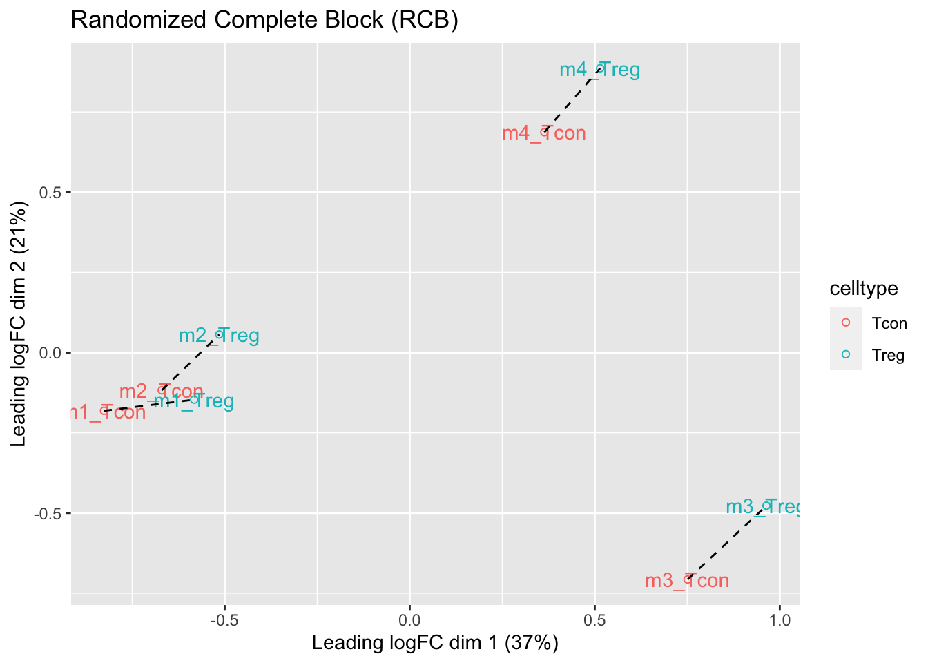
• We observe that the leading fold change is according to mouse

• In the second dimension we see a separation according to cell-type

• With the Randomized Complete Block design (RCB) we can remove the mouse effect from the analysis!

• We can isolate the between block variability from the analysis using linear model:

  • Formula in R \[ y \sim \text{celltype} + \text{mouse} \]

  • Formula

\[ y_i = \beta_0 + \beta_\text{Treg} x_{i,\text{Treg}} + \beta_{m2}x_{i,m2} + \beta_{m3}x_{i,m3} + \beta_{m4}x_{i,m4} + \epsilon_i \]

with

• \(x_{i,Treg}=\begin{cases} 1& \text{Treg}\\ 0& \text{Tcon} \end{cases}\)

• \(x_{i,m2}=\begin{cases} 1& \text{m2}\\ 0& \text{otherwise} \end{cases}\)

• \(x_{i,m3}=\begin{cases} 1& \text{m3}\\ 0& \text{otherwise} \end{cases}\)

• \(x_{i,m4}=\begin{cases} 1& \text{m4}\\ 0& \text{otherwise} \end{cases}\)

• Possible in msqrob2 and MSstats but not possible with Perseus!

3.3 Modeling and inference

3.3.1 RCB analysis

pe <- msqrob(
  object = pe,
  i = "protein",
  formula = ~ celltype + mouse)

3.3.2 CRD analysis

pe2 <- msqrob(
  object = pe2,
  i = "protein",
  formula = ~ celltype)

3.3.3 Estimation, effect size and inference

Effect size in RCB

library(ExploreModelMatrix)
VisualizeDesign(colData(pe),~ celltype + mouse)$plotlist

## [[1]]

Effect size in CRD

VisualizeDesign(colData(pe2),~ celltype)$plotlist

## [[1]]

Click to see code for statistical inference

L <- makeContrast("celltypeTreg = 0", parameterNames = c("celltypeTreg"))
pe <- hypothesisTest(object = pe, i = "protein", contrast = L)
pe2 <- hypothesisTest(object = pe2, i = "protein", contrast = L)

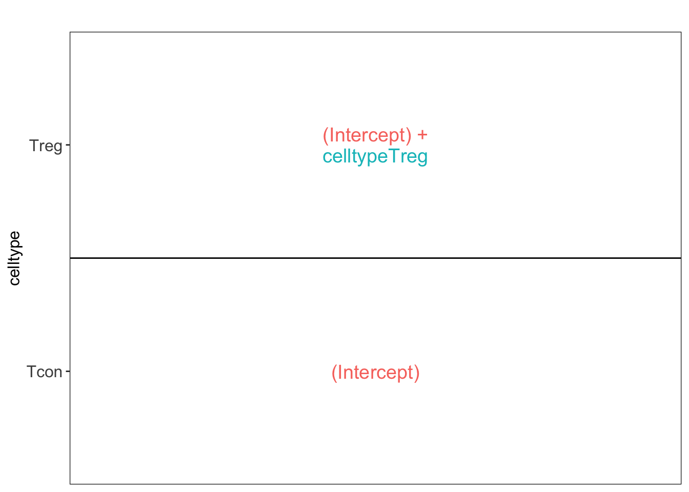
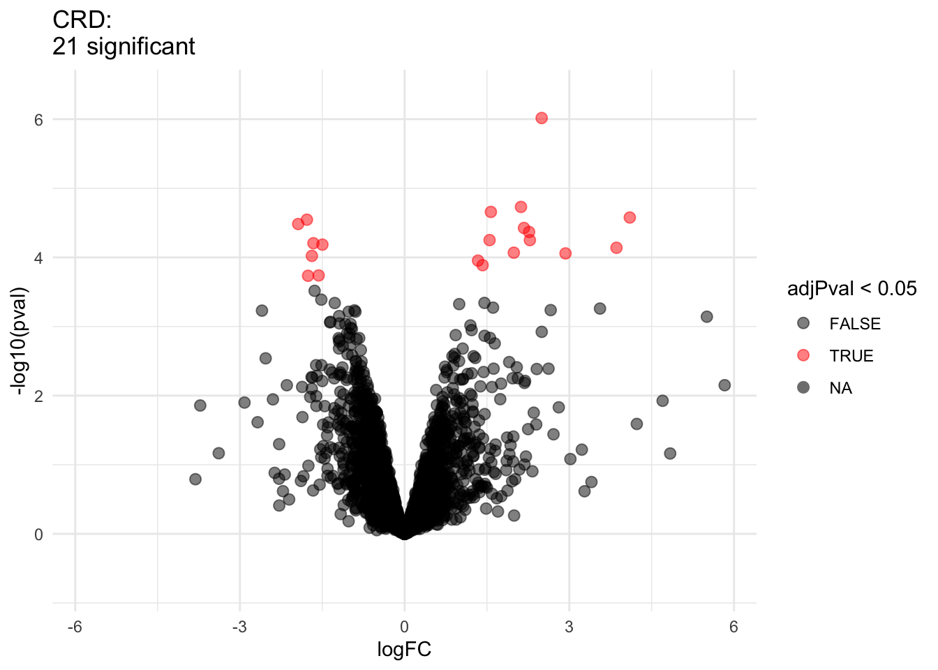
3.3.4 Comparison of results

Click to see code

3.3.5 Comparison of standard deviation

Click to see code

accessions <- rownames(pe[["protein"]])[rownames(pe[["protein"]])%in%rownames(pe2[["protein"]])]
dat <- data.frame(
sigmaRBC = sapply(rowData(pe[["protein"]])$msqrobModels[accessions], getSigmaPosterior),
sigmaCRD <- sapply(rowData(pe2[["protein"]])$msqrobModels[accessions], getSigmaPosterior)
)

plotRBCvsCRD <- ggplot(data = dat, aes(sigmaRBC, sigmaCRD)) +
    geom_point(alpha = 0.1, shape = 20) +
    scale_x_log10() +
    scale_y_log10() +
    geom_abline(intercept=0,slope=1)

  plotRBCvsCRD

## Warning: Removed 743 rows containing missing values (geom_point).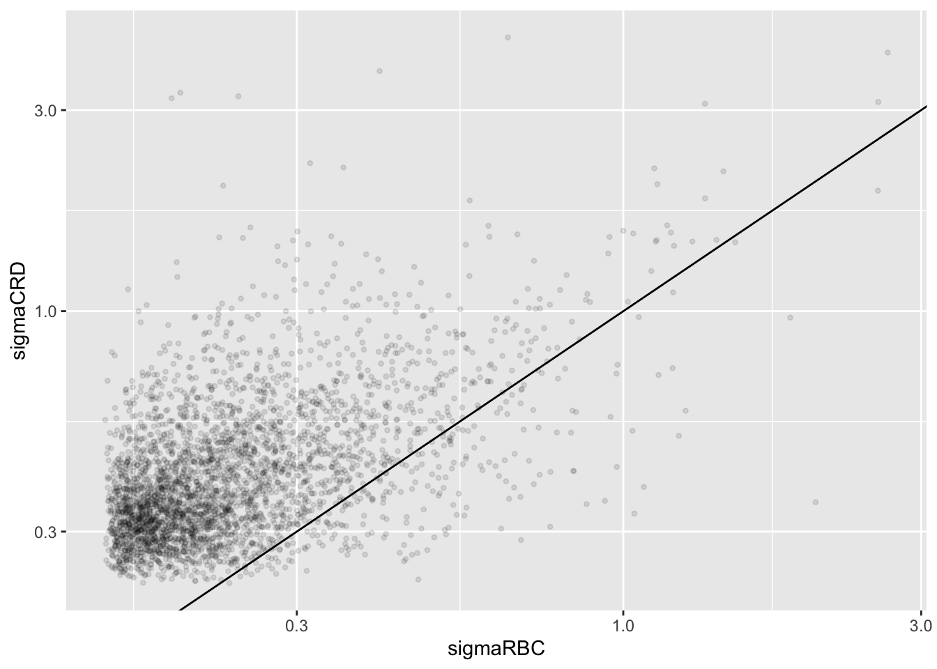

• We clearly observe that the standard deviation of the protein expression in the RCB is smaller for the majority of the proteins than that obtained with the CRD

• Why are some of the standard deviations for the RCB with the correct analysis larger than than of the RCB with the incorrect analysis that ignored the mouse blocking factor?

• Can you think of a reason why it would not be useful to block on a particular factor?