Statistical Methods for Quantitative MS-based Proteomics: Part II. Differential Abundance Analysis

This is part of the online course Proteomics Data Analysis 2021 (PDA21)

• Playlist PDA Preprocessing

Outline

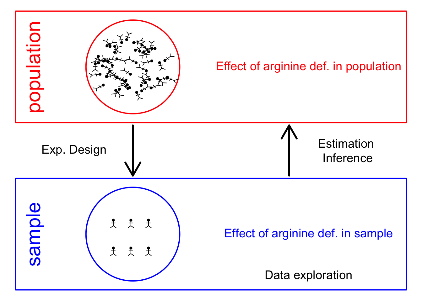
• Francisella tularensis Example
• Hypothesis testing
• Multiple testing
• Moderated statistics
• Experimental design

Note, that the R-code is included for learners who are aiming to develop R/markdown scripts to automate their quantitative proteomics data analyses. According to the target audience of the course we either work with a graphical user interface (GUI) in a R/shiny App msqrob2gui (e.g. Proteomics Bioinformatics course of the EBI and the Proteomics Data Analysis course at the Gulbenkian institute) or with R/markdowns scripts (e.g. Bioinformatics Summer School at UCLouvain or the Statistical Genomics Course at Ghent University).

---

1 Francisella tularensis experiment

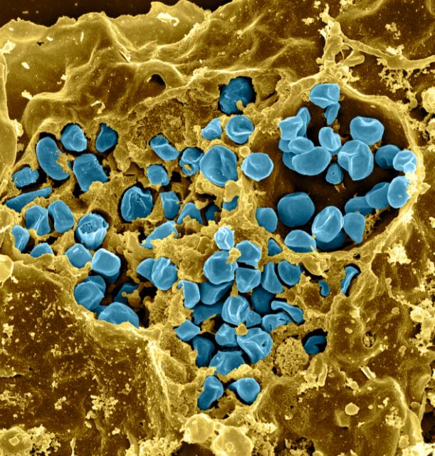
• Pathogen: causes tularemia
• Metabolic adaptation key for intracellular life cycle of pathogenic microorganisms.
• Upon entry into host cells quick phasomal escape and active multiplication in cytosolic compartment.
• Franciscella is auxotroph for several amino acids, including arginine.
• Inactivation of arginine transporter delayed bacterial phagosomal escape and intracellular multiplication.
• Experiment to assess difference in proteome using 3 WT vs 3 ArgP KO mutants

1.1 Import the data in R

Click to see code

1. Load libraries

library(tidyverse)
library(limma)
library(QFeatures)
library(msqrob2)
library(plotly)
library(ggplot2)

2. We use a peptides.txt file from MS-data quantified with maxquant that contains MS1 intensities summarized at the peptide level.

peptidesFile <- "https://raw.githubusercontent.com/statOmics/PDA21/data/quantification/francisella/peptides.txt"

3. Maxquant stores the intensity data for the different samples in columnns that start with Intensity. We can retreive the column names with the intensity data with the code below:

ecols <- grep("Intensity\\.", names(read.delim(peptidesFile)))

4. Read the data and store it in QFeatures object

pe <- readQFeatures(
  table = peptidesFile,
  fnames = 1,
  ecol = ecols,
  name = "peptideRaw", sep="\t")

5. Update data with information on design

colData(pe)$genotype <- pe[[1]] %>% 
  colnames %>% 
  substr(12,13) %>%
  as.factor %>% 
  relevel("WT")
pe %>% colData

## DataFrame with 6 rows and 1 column
##                          genotype
##                          <factor>
## Intensity.1WT_20_2h_n3_3       WT
## Intensity.1WT_20_2h_n4_3       WT
## Intensity.1WT_20_2h_n5_3       WT
## Intensity.3D8_20_2h_n3_3       D8
## Intensity.3D8_20_2h_n4_3       D8
## Intensity.3D8_20_2h_n5_3       D8

1.2 Preprocessing

Click to see code to log-transfrom the data

1. Log transform

• Calculate number of non zero intensities for each peptide

rowData(pe[["peptideRaw"]])$nNonZero <- rowSums(assay(pe[["peptideRaw"]]) > 0)

• Peptides with zero intensities are missing peptides and should be represent with a NA value rather than 0.

pe <- zeroIsNA(pe, "peptideRaw") # convert 0 to NA

• Logtransform data with base 2

pe <- logTransform(pe, base = 2, i = "peptideRaw", name = "peptideLog")

2. Filtering

• Handling overlapping protein groups

pe <- filterFeatures(pe, ~ Proteins %in% smallestUniqueGroups(rowData(pe[["peptideLog"]])$Proteins))

• Remove reverse sequences (decoys) and contaminants. Note that this is indicated by the column names Reverse and depending on the version of maxQuant with Potential.contaminants or Contaminants.

pe <- filterFeatures(pe,~Reverse != "+")
pe <- filterFeatures(pe,~ Contaminant != "+")

• Drop peptides that were only identified in one sample

pe <- filterFeatures(pe,~ nNonZero >=2)
nrow(pe[["peptideLog"]])

## [1] 6525

We keep 6525 peptides upon filtering.

3. Normalization by median centering

pe <- normalize(pe, 
                i = "peptideLog", 
                name = "peptideNorm", 
                method = "center.median")

4. Summarization. We use the standard sumarisation in aggregateFeatures, which is a robust summarisation method.

pe <- aggregateFeatures(pe,
    i = "peptideNorm", 
    fcol = "Proteins", 
    na.rm = TRUE,
    name = "protein")

## Your quantitative and row data contain missing values. Please read the
## relevant section(s) in the aggregateFeatures manual page regarding the
## effects of missing values on data aggregation.

Plot of preprocessed data

pe[["peptideNorm"]] %>% 
  assay %>%
  as.data.frame() %>%
  gather(sample, intensity) %>% 
  mutate(genotype = colData(pe)[sample,"genotype"]) %>%
  ggplot(aes(x = intensity,group = sample,color = genotype)) + 
    geom_density() +
    ggtitle("Peptide-level")

## Warning: Removed 7561 rows containing non-finite values (stat_density).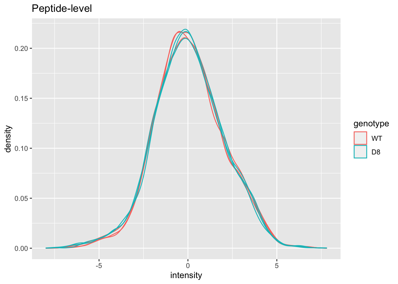

pe[["protein"]] %>% 
  assay %>%
  as.data.frame() %>%
  gather(sample, intensity) %>% 
  mutate(genotype = colData(pe)[sample,"genotype"]) %>%
  ggplot(aes(x = intensity,group = sample,color = genotype)) + 
    geom_density() +
    ggtitle("Protein-level")

## Warning: Removed 428 rows containing non-finite values (stat_density).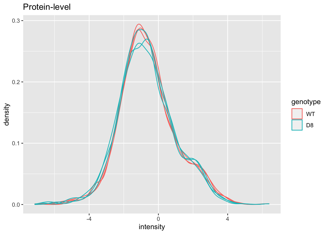

1.3 Summarized data structure

1.3.1 Design

pe %>% 
  colData %>% 
  knitr::kable()

	genotype
Intensity.1WT_20_2h_n3_3	WT
Intensity.1WT_20_2h_n4_3	WT
Intensity.1WT_20_2h_n5_3	WT
Intensity.3D8_20_2h_n3_3	D8
Intensity.3D8_20_2h_n4_3	D8
Intensity.3D8_20_2h_n5_3	D8

• WT vs KO
• 3 vs 3 repeats

1.3.2 Summarized intensity matrix

pe[["protein"]] %>% assay() %>% head() %>% knitr::kable()

	Intensity.1WT_20_2h_n3_3	Intensity.1WT_20_2h_n4_3	Intensity.1WT_20_2h_n5_3	Intensity.3D8_20_2h_n3_3	Intensity.3D8_20_2h_n4_3	Intensity.3D8_20_2h_n5_3
WP_003013731	-0.2748775	-0.0856247	0.1595370	-0.2809009	0.0035526	0.0567110
WP_003013860	NA	NA	-0.2512039	NA	NA	-0.4865646
WP_003013909	-0.6851118	-0.8161658	-0.7557906	-0.4591476	-0.5449424	-0.4962482
WP_003014068	0.6495386	0.8522239	1.1344852	0.5459176	0.9187714	0.5974741
WP_003014122	-0.7630863	-1.0430741	-0.8091715	-1.1743951	-1.1924725	-1.2565893
WP_003014123	-0.2051672	-0.3361704	-0.2151930	-0.3855747	-0.2802011	-0.5801771

• 1115 proteins

1.3.3 Hypothesis testing: a single protein

1.3.3.1 T-test

\[ \log_2 \text{FC} = \bar{y}_{p1}-\bar{y}_{p2} \]

\[ T_g=\frac{\log_2 \text{FC}}{\text{se}_{\log_2 \text{FC}}} \]

\[ T_g=\frac{\widehat{\text{signal}}}{\widehat{\text{Noise}}} \]

If we can assume equal variance in both treatment groups:

\[ \text{se}_{\log_2 \text{FC}}=\text{SD}\sqrt{\frac{1}{n_1}+\frac{1}{n_2}} \]

WP_003023392 <- data.frame(
    intensity = assay(pe[["protein"]]["WP_003023392",]) %>% c(), 
    genotype = colData(pe)[,1]) 

WP_003023392 %>% 
  ggplot(aes(x=genotype,y=intensity)) + 
  geom_point() +
  ggtitle("Protein WP_003023392")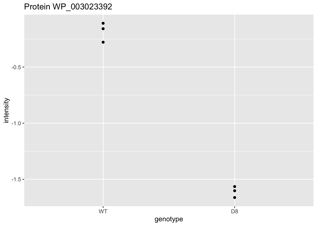

\[ t=\frac{\log_2\widehat{\text{FC}}}{\text{se}_{\log_2\widehat{\text{FC}}}}=\frac{-1.43}{0.0577}=-24.7 \]

• Is t = -24.7 indicating that there is an effect?

• How likely is it to observe t = -24.7 when there is no effect of the argP KO on the protein expression?

1.3.3.2 Null hypothesis (\(H_0\)) and alternative hypothesis (\(H_1\))

• With data we can never prove a hypothesis (falsification principle of Popper)

• With data we can only reject a hypothesis

• In general we start from alternative hypothese \(H_1\): we want to show an effect of the KO on a protein

\(H_1\): On average the protein abundance in WT is different from that in KO

• But, we will assess this by falsifying the opposite: \(H_0\): On average the protein abundance in WT is equal to that in KO<-

t.test(intensity ~ genotype, data = WP_003023392, var.equal=TRUE)

## 
##  Two Sample t-test
## 
## data:  intensity by genotype
## t = 24.747, df = 4, p-value = 1.582e-05
## alternative hypothesis: true difference in means between group WT and group D8 is not equal to 0
## 95 percent confidence interval:
##  1.267666 1.588058
## sample estimates:
## mean in group WT mean in group D8 
##       -0.1821147       -1.6099769

• How likely is it to observe an equal or more extreme effect than the one observed in the sample when the null hypothesis is true?

• When we make assumptions about the distribution of our test statistic we can quantify this probability: p-value. The p-value will only be calculated correctly if the underlying assumptions hold!

• When we repeat the experiment, the probability to observe a fold change for this gene that is more extreme than a 2.69 fold (\(\log_2 FC=-1.43\)) down or up regulation by random change (if \(H_0\) is true) is 16 out of 1 000 000.
  

• If the p-value is below a significance threshold \(\alpha\) we reject the null hypothesis. We control the probability on a false positive result at the \(\alpha\)-level (type I error)

• Note, that the p-values are uniform under the null hypothesis, i.e. when \(H_0\) is true all p-values are equally likely.

1.4 Multiple hypothesis testing

• Consider testing DA for all \(m=1066\) proteins simultaneously

• What if we assess each individual test at level \(\alpha\)? \(\rightarrow\) Probability to have a false positive (FP) among all m simultatenous test \(>>> \alpha= 0.05\)

• Indeed for each non DA protein we have a probability of 5% to return a FP.

• In a typical experiment the majority of the proteins are non DA.

• So an upperbound of the expected FP is \(m \times \alpha\) or \(1066 \times 0.05=53\).

\(\rightarrow\) Hence, we are bound to call many false positive proteins each time we run the experiment.

1.4.1 Multiple testing

1.4.1.1 Family-wise error rate

The family-wise error rate (FWER) addresses the multiple testing issue by no longer controlling the individual type I error for each protein, instead it controls:

\[ \text{FWER} = \text{P}\left[FP \geq 1 \right]. \]

The Bonferroni method is widely used to control the type I error:

• assess each test at \[\alpha_\text{adj}=\frac{\alpha}{m}\]
• or use adjusted p-values and compare them to \(\alpha\): \[p_\text{adj}=\text{min}\left(p \times m,1\right)\]

Problem, the method is very conservative!

1.4.1.2 False discovery rate

• FDR: Expected proportion of false positives on the total number of positives you return.
• An FDR of 1% means that on average we expect 1% false positive proteins in the list of proteins that are called significant.
• Defined by Benjamini and Hochberg in their seminal paper Benjamini, Y. and Hochberg, Y. (1995). “Controlling the false discovery rate: a practical and powerful approach to multiple testing”. Journal of the Royal Statistical Society Series B, 57 (1): 289–300.

The False Discovery Proportion (FDP) is the fraction of false positives that are returned, i.e. 

\[ FDP = \frac{FP}{R} \]

• However, this quantity cannot be observed because in practice we only know the number of proteins for which we rejected \(H_0\), \(R\).
• But, we do not know the number of false positives, \(FP\).

Therefore, Benjamini and Hochberg, 1995, defined The False Discovery Rate (FDR) as \[ \text{FDR} = \text{E}\left[\frac{FP}{R}\right] =\text{E}\left[\text{FDP}\right] \] the expected FDP.

• Controlling the FDR allows for more discoveries (i.e. longer lists with significant results), while the fraction of false discoveries among the significant results in well controlled on average. As a consequence, more of the true positive hypotheses will be detected.

1.4.1.3 Intuition of BH-FDR procedure

Consider \(m = 1000\) tests

• Suppose that a researcher rejects all null hypotheses for which \(p < 0.01\).

• If we use \(p < 0.01\), we expect \(0.01 \times m_0\) tests to return false positives.

• A conservative estimate of the number of false positives that we can expect can be obtained by considering that the null hypotheses are true for all features, \(m_0 = m = 1000\).

• We then would expect \(0.01 \times 1000 = 10\) false positives (\(FP=10\)).

• Suppose that the researcher found 200 genes with \(p<0.01\) (\(R=200\)).

• The proportion of false positive results (FDP = false positive proportion) among the list of \(R=200\) genes can then be estimated as \[ \widehat{\text{FDP}}=\frac{FP}{R}=\frac{10}{200}=\frac{0.01 \times 1000}{200} = 0.05. \]

1.4.1.4 Benjamini and Hochberg (1995) procedure for controlling the FDR at \(\alpha\)

1. Let \(p_{(1)}\leq \ldots \leq p_{(m)}\) denote the ordered \(p\)-values.

2. Find the largest integer \(k\) so that \[ \frac{p_{(k)} \times m}{k} \leq \alpha \] \[\text{or}\] \[ p_{(k)} \leq k \times \alpha/m \]

3. If such a \(k\) exists, reject the \(k\) null hypotheses associated with \(p_{(1)}, \ldots, p_{(k)}\). Otherwise none of the null hypotheses is rejected.

The adjusted \(p\)-value (also known as the \(q\)-value in FDR literature): \[ q_{(i)}=\tilde{p}_{(i)} = \min\left[\min_{j=i,\ldots, m}\left(m p_{(j)}/j\right), 1 \right]. \] In the hypothetical example above: \(k=200\), \(p_{(k)}=0.01\), \(m=1000\) and \(\alpha=0.05\).

1.4.1.5 Francisella Example

Click to see code

ttestMx <- function(y,group) {
    test <- try(t.test(y[group],y[!group],var.equal=TRUE),silent=TRUE)
    if(is(test,"try-error")) {
      return(c(log2FC=NA,se=NA,tstat=NA,p=NA))
      } else {
      return(c(log2FC= (test$estimate%*%c(1,-1)),se=test$stderr,tstat=test$statistic,pval=test$p.value))
      }
 }
 
 res <- apply(
    assay(pe[["protein"]]), 
    1, 
    ttestMx,
    group = colData(pe)$genotype=="D8") %>% 
  t 
 colnames(res) <- c("logFC","se","tstat","pval")
 res <- res %>% as.data.frame %>% na.exclude %>% arrange(pval)
 res$adjPval <- p.adjust(res$pval, "fdr")
 alpha <- 0.05
res$adjAlphaForm <- paste0(1:nrow(res)," x ",alpha,"/",nrow(res))
res$adjAlpha <- alpha * (1:nrow(res))/nrow(res) 
res$"pval < adjAlpha" <- res$pval < res$adjAlpha 
res$"adjPval < alpha" <- res$adjPval < alpha 

FWER: Bonferroni method:\(\alpha_\text{adj} = \alpha/m = 0.05 / 1066= 5\times 10^{-5}\)

	logFC	pval	adjPval	adjAlphaForm	adjAlpha	pval < adjAlpha	adjPval < alpha
WP_003038940	-0.2876290	0.0000146	0.0084347	1 x 0.05/1066	0.0000469	TRUE	TRUE
WP_003023392	-1.4278622	0.0000158	0.0084347	2 x 0.05/1066	0.0000938	TRUE	TRUE
WP_003039212	-0.2658247	0.0000820	0.0291520	3 x 0.05/1066	0.0001407	TRUE	TRUE
WP_003026016	-1.0800305	0.0001395	0.0346124	4 x 0.05/1066	0.0001876	TRUE	TRUE
WP_003039615	-0.3992190	0.0001623	0.0346124	5 x 0.05/1066	0.0002345	TRUE	TRUE
WP_011733588	-0.4323262	0.0002291	0.0407034	6 x 0.05/1066	0.0002814	TRUE	TRUE
WP_003014552	-0.9843865	0.0003224	0.0440266	7 x 0.05/1066	0.0003283	TRUE	TRUE
WP_003040849	-1.2780743	0.0003304	0.0440266	8 x 0.05/1066	0.0003752	TRUE	TRUE
WP_003038430	-0.4331987	0.0004505	0.0489078	9 x 0.05/1066	0.0004221	FALSE	TRUE
WP_003033975	-0.2949061	0.0005047	0.0489078	10 x 0.05/1066	0.0004690	FALSE	TRUE
WP_011733645	0.3531405	0.0005171	0.0489078	11 x 0.05/1066	0.0005159	FALSE	TRUE
WP_011733723	-0.3935768	0.0005506	0.0489078	12 x 0.05/1066	0.0005629	TRUE	TRUE
WP_003038679	-0.3909725	0.0007083	0.0580821	13 x 0.05/1066	0.0006098	FALSE	FALSE
WP_003033719	-1.1865453	0.0008426	0.0603810	14 x 0.05/1066	0.0006567	FALSE	FALSE
…	…	…	…	…	…	…	…
WP_003040562	0.0039480	0.9976429	0.9985797	1065 x 0.05/1066	0.0499531	FALSE	FALSE
WP_003041130	0.0002941	0.9992812	0.9992812	1066 x 0.05/1066	0.05	FALSE	FALSE

1.4.1.6 Results

Click to see code

volcanoT <- res %>% 
  ggplot(aes(x = logFC, y = -log10(pval), color = adjPval < 0.05)) +
    geom_point(cex = 2.5) +
    scale_color_manual(values = alpha(c("black", "red"), 0.5)) +
    theme_minimal() 

volcanoT

1.5 Moderated Statistics

Problems with ordinary t-test

Click to see code

problemPlots <- list() 
problemPlots[[1]] <- res %>% 
  ggplot(aes(x = logFC, y = se, color = adjPval < 0.05)) +
    geom_point(cex = 2.5) +
    scale_color_manual(values = alpha(c("black", "red"), 0.5)) +
    theme_minimal() 

for (i in 2:3)
{
problemPlots[[i]] <- colData(pe) %>% 
    as.data.frame %>% 
    mutate(intensity = pe[["protein"]][rownames(res)[i],] %>% 
             assay %>% 
             c) %>% 
    ggplot(aes(x=genotype,y=intensity)) +
    geom_point() + 
    ylim(-3,0) +
    ggtitle(rownames(res)[i])
}

problemPlots

## [[1]]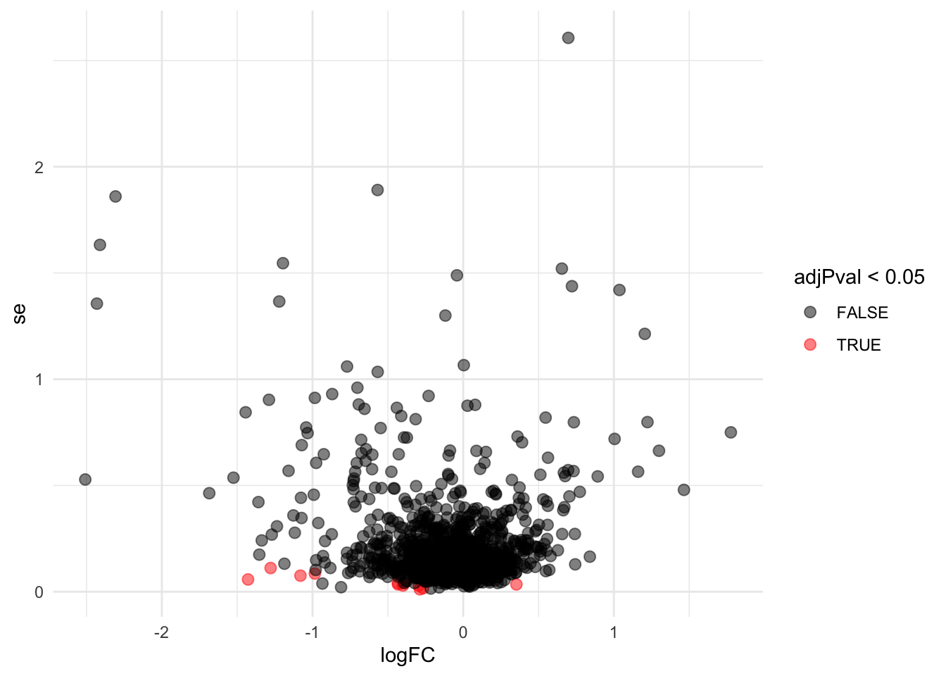

## 
## [[2]]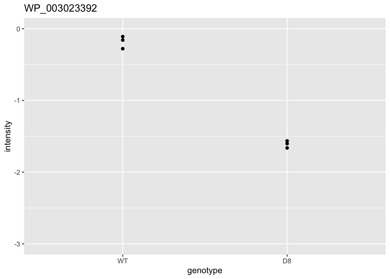

## 
## [[3]]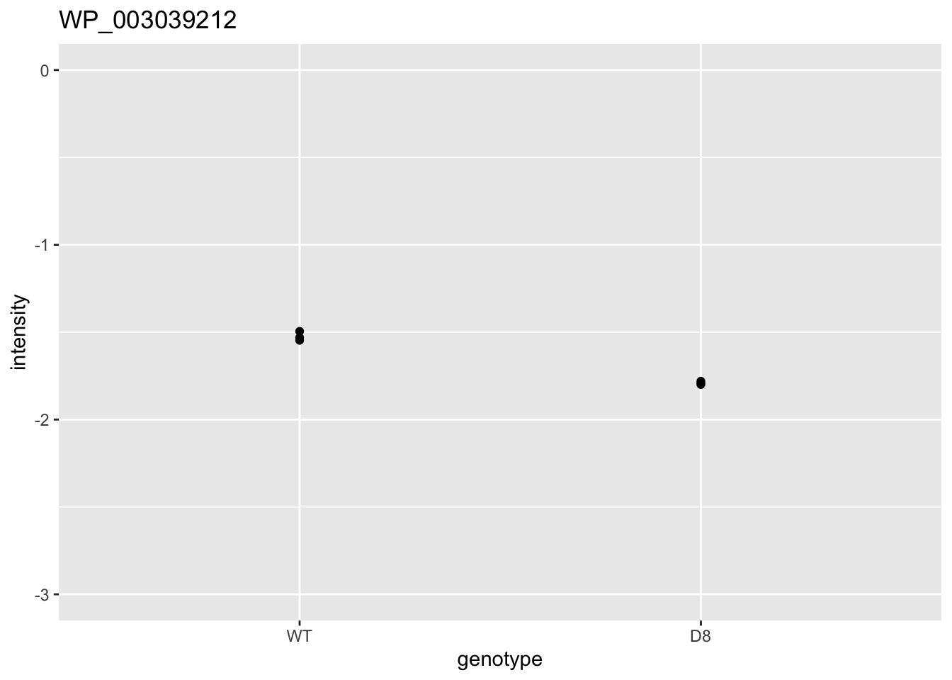

A general class of moderated test statistics is given by \[ T_g^{mod} = \frac{\bar{Y}_{g1} - \bar{Y}_{g2}}{C \quad \tilde{S}_g} , \] where \(\tilde{S}_g\) is a moderated standard deviation estimate.

• \(C\) is a constant depending on the design e.g. \(\sqrt{1/{n_1}+1/n_2}\) for a t-test and of another form for linear models.
• \(\tilde{S}_g=S_g+S_0\): add small positive constant to denominator of t-statistic.
• This can be adopted in Perseus.

Click to see code

simI<-sapply(res$se/sqrt(1/3+1/3),function(n,mean,sd) rnorm(n,mean,sd),n=6,mean=0) %>% t
resSim <- apply(
    simI, 
    1, 
    ttestMx,
    group = colData(pe)$genotype=="D8") %>% 
  t 
 colnames(resSim) <- c("logFC","se","tstat","pval")
 resSim <- as.data.frame(resSim)
 tstatSimPlot <- resSim %>% 
   ggplot(aes(x=tstat)) +
     geom_histogram(aes(y=..density.., fill=..count..),bins=30) +
     stat_function(fun=dt,
    color="red",
    args=list(df=4)) + 
   ylim(0,.6) +
   ggtitle("t-statistic")

 
 resSim$C <- sqrt(1/3+1/3) 
 resSim$sd <- resSim$se/resSim$C 
 tstatSimPerseus <- resSim %>% 
   ggplot(aes(x=logFC/((sd+.1)*C))) +
     geom_histogram(aes(y=..density.., fill=..count..),bins=30) +
     stat_function(fun=dt,
                   color="red",
                  args=list(df=4)) + 
     ylim(0,.6) +
    ggtitle("Perseus")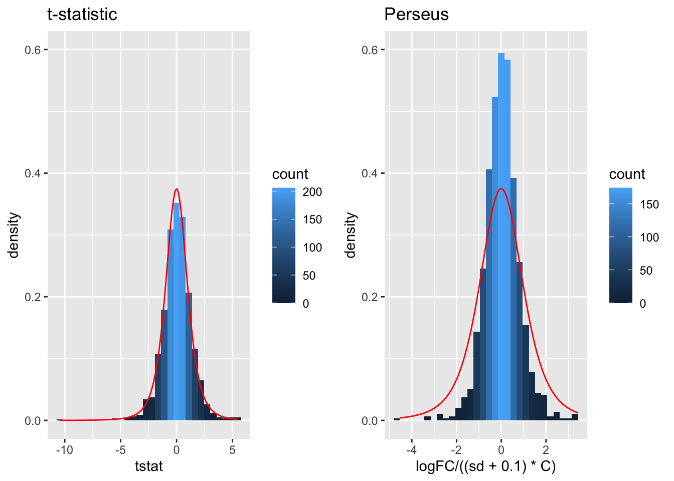

gridExtra::grid.arrange(tstatSimPlot,tstatSimPerseus,nrow=1)

• The choice of \(S_0\) in Perseus is ad hoc and the t-statistic is no-longer t-distributed.
• Permutation test, but is difficult for more complex designs.
• Allows for Data Dredging because user can choose \(S_0\)

1.5.1 Empirical Bayes

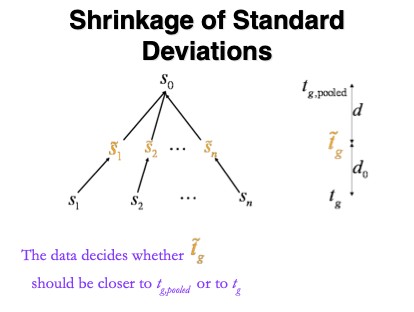
Figure courtesy to Rafael Irizarry

\[ T_g^{mod} = \frac{\bar{Y}_{g1} - \bar{Y}_{g2}}{C \quad \tilde{S}_g} , \]

• empirical Bayes theory provides formal framework for borrowing strength across proteins,
• Implemented in popular bioconductor package limma and msqrob2

\[ \tilde{S}_g=\sqrt{\frac{d_gS_g^2+d_0S_0^2}{d_g+d_0}}, \]

• \(S_0^2\): common variance (over all proteins)
• Moderated t-statistic is t-distributed with \(d_0+d_g\) degrees of freedom.
• Note that the degrees of freedom increase by borrowing strength across proteins!

Click to see the code

1. We model the protein level expression values using the msqrob function. By default msqrob2 estimates the model parameters using robust regression.

We will model the data with a different group mean for every genotype. The group is incoded in the variable genotype of the colData. We can specify this model by using a formula with the factor genotype as its predictor: formula = ~genotype.

Note, that a formula always starts with a symbol ‘~’.

pe <- msqrob(object = pe, i = "protein", formula = ~genotype)

2. Inference

We first explore the design of the model that we specified using the the package ExploreModelMatrix

library(ExploreModelMatrix)
VisualizeDesign(colData(pe),~genotype)$plotlist[[1]]

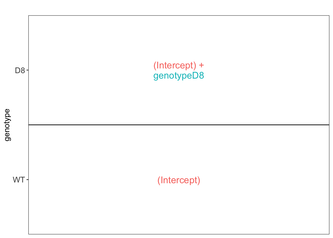
We have two model parameters, the (Intercept) and genotypeD8. This results in a model with two group means:

1. For the wild type (WT) the expected value (mean) of the log2 transformed intensity y for a protein will be modelled using

\[\text{E}[Y\vert \text{genotype}=\text{WT}] = \text{(Intercept)}\]

2. For the knockout genotype D8 the expected value (mean) of the log2 transformed intensity y for a protein will be modelled using

\[\text{E}[Y\vert \text{genotype}=\text{D8}] = \text{(Intercept)} + \text{genotypeD8}\]

The average log2FC between D8 and WT is thus \[\log_2\text{FC}_{D8-WT}= \text{E}[Y\vert \text{genotype}=\text{D8}] - \text{E}[Y\vert \text{genotype}=\text{WT}] = \text{genotypeD8} \]

Hence, assessing the null hypothesis that there is no differential abundance between D8 and WT can be reformulated as

\[H_0: \text{genotypeD8}=0\] We can implement a hypothesis test for each protein in msqrob2 using the code below:

L <- makeContrast("genotypeD8 = 0", parameterNames = c("genotypeD8"))
pe <- hypothesisTest(object = pe, i = "protein", contrast = L)

We can show the list with all significant DE proteins at the 5% FDR using

rowData(pe[["protein"]])$genotypeD8 %>% 
  arrange(pval) %>%
  filter(adjPval<0.05)

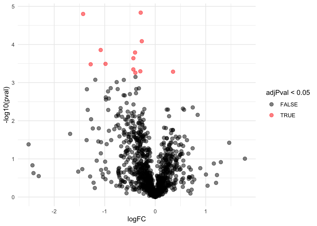
We can also visualise the results using a volcanoplot

volcano <- ggplot(
    rowData(pe[["protein"]])$genotypeD8,
    aes(x = logFC, y = -log10(pval), color = adjPval < 0.05)
) +
    geom_point(cex = 2.5) +
    scale_color_manual(values = alpha(c("black", "red"), 0.5)) +
    theme_minimal() +
    ggtitle("msqrob2")

gridExtra::grid.arrange(
  volcanoT +    
    xlim(-3,3) +
  ggtitle("ordinary t-test"),
  volcano +     
    xlim(-3,3)
,nrow=2)

## Warning: Removed 109 rows containing missing values (geom_point).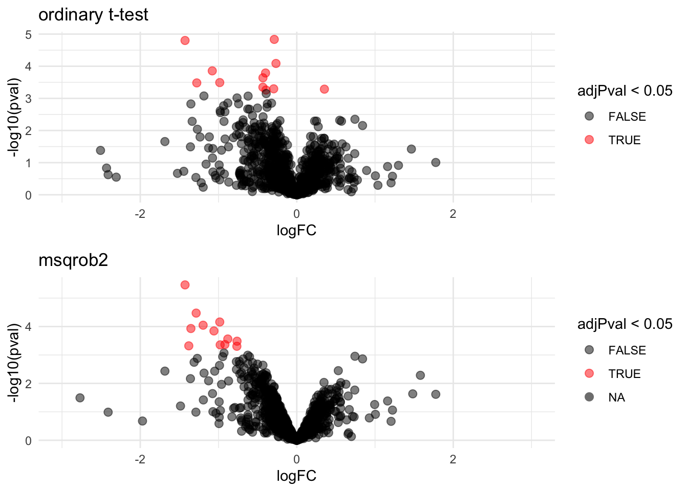

• The volcano plot opens up when using the EB variance estimator

• Borrowing strength to estimate the variance using empirical Bayes solves the issue of returning proteins with a low fold change as significant due to a low variance.

1.5.2 Shrinkage of the variance and moderated t-statistics

qplot(
  sapply(rowData(pe[["protein"]])$msqrobModels,getSigma),
  sapply(rowData(pe[["protein"]])$msqrobModels,getSigmaPosterior)) +
  xlab("SD") +
  ylab("moderated SD") +
  geom_abline(intercept = 0,slope = 1) +
  geom_hline(yintercept = ) 

## Warning: Removed 109 rows containing missing values (geom_point).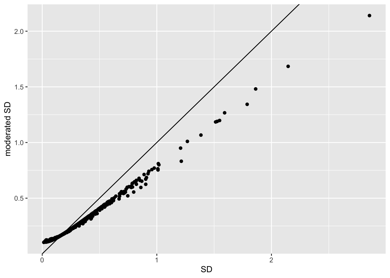

• Small variances are shrunken towards the common variance resulting in large EB variance estimates
• Large variances are shrunken towards the common variance resulting in smaller EB variance estimates
• Pooled degrees of freedom of the EB variance estimator are larger because information is borrowed across proteins to estimate the variance

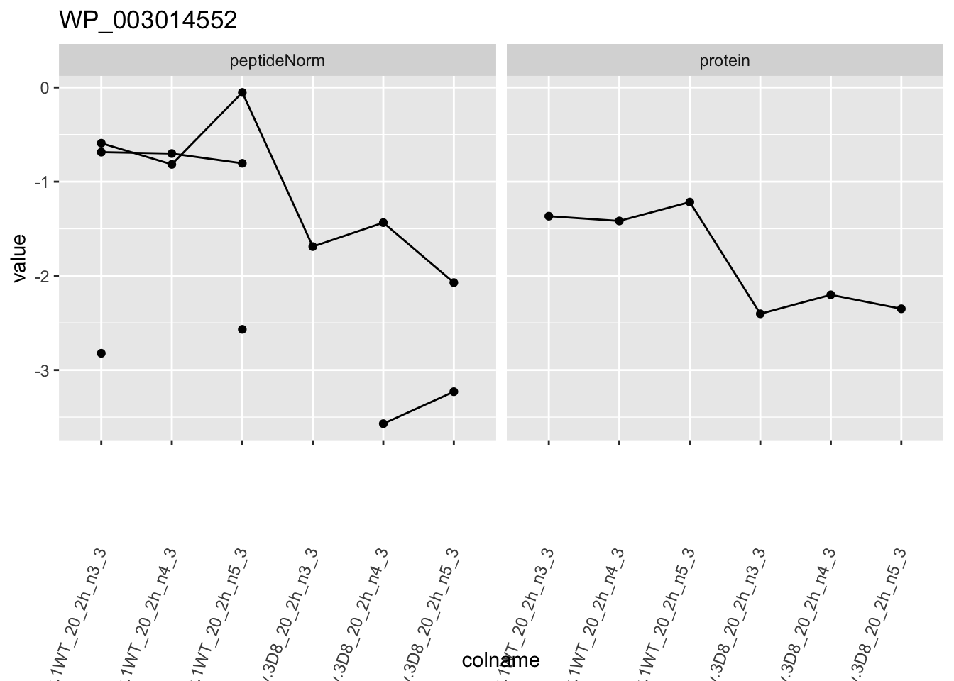
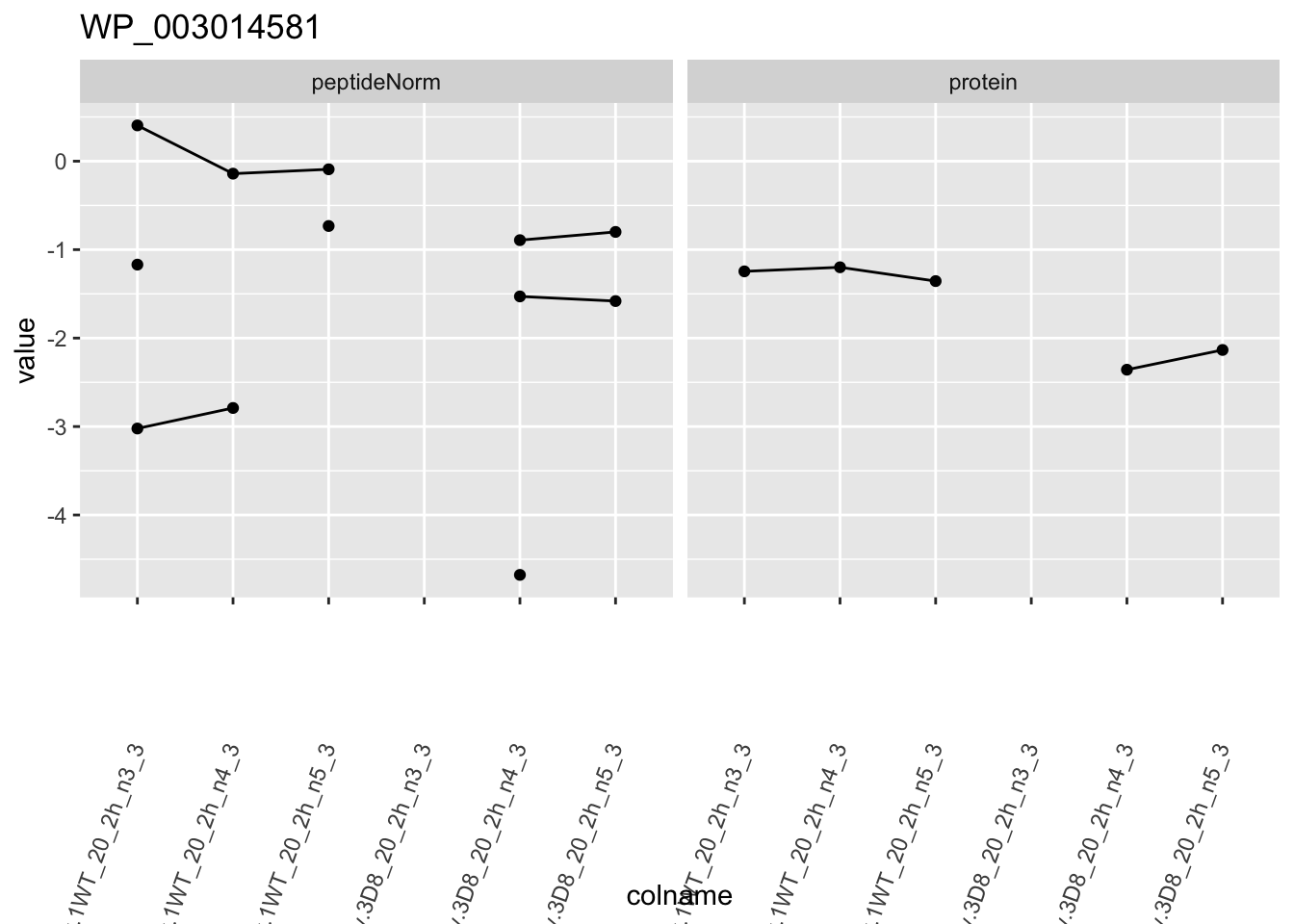
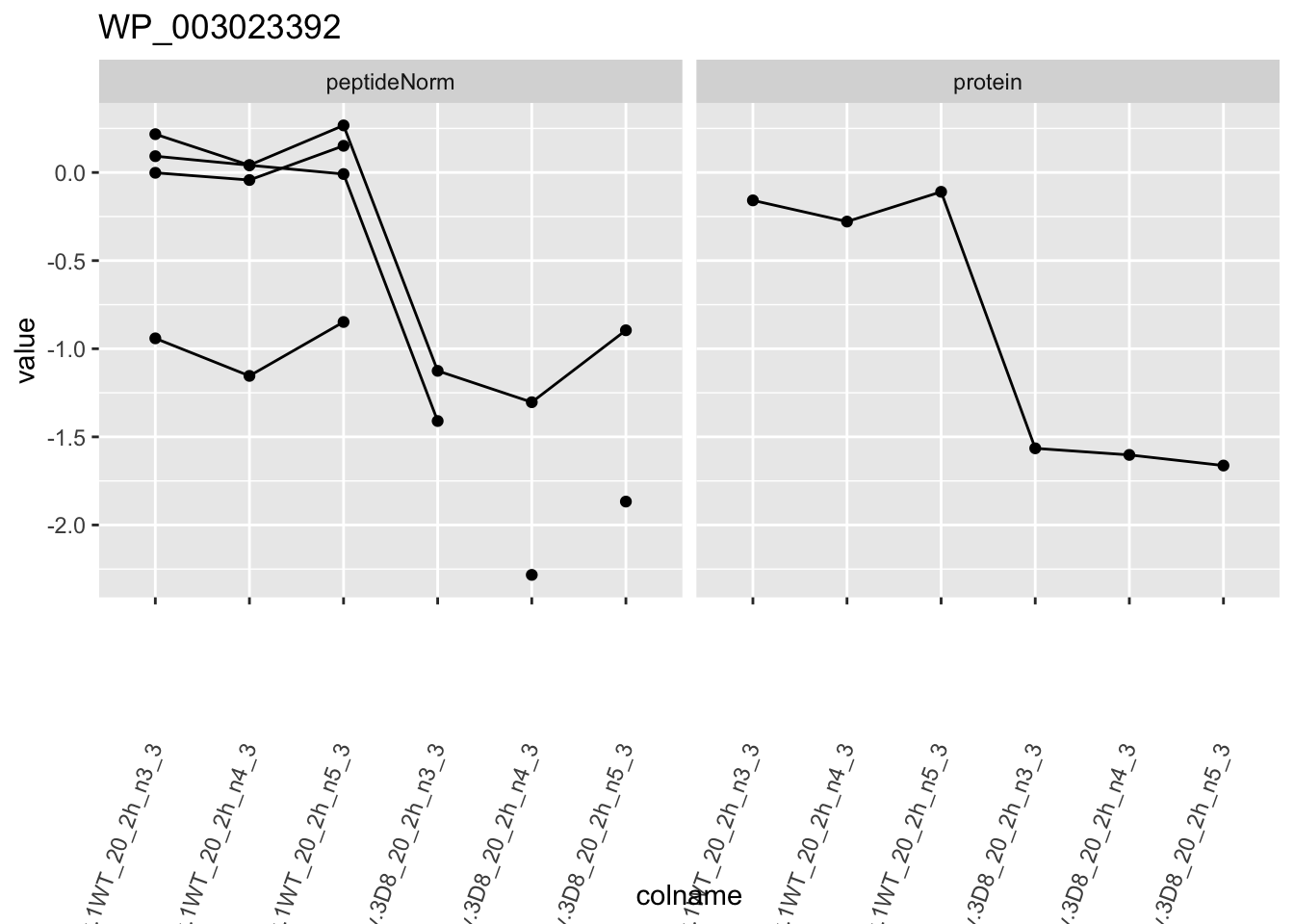
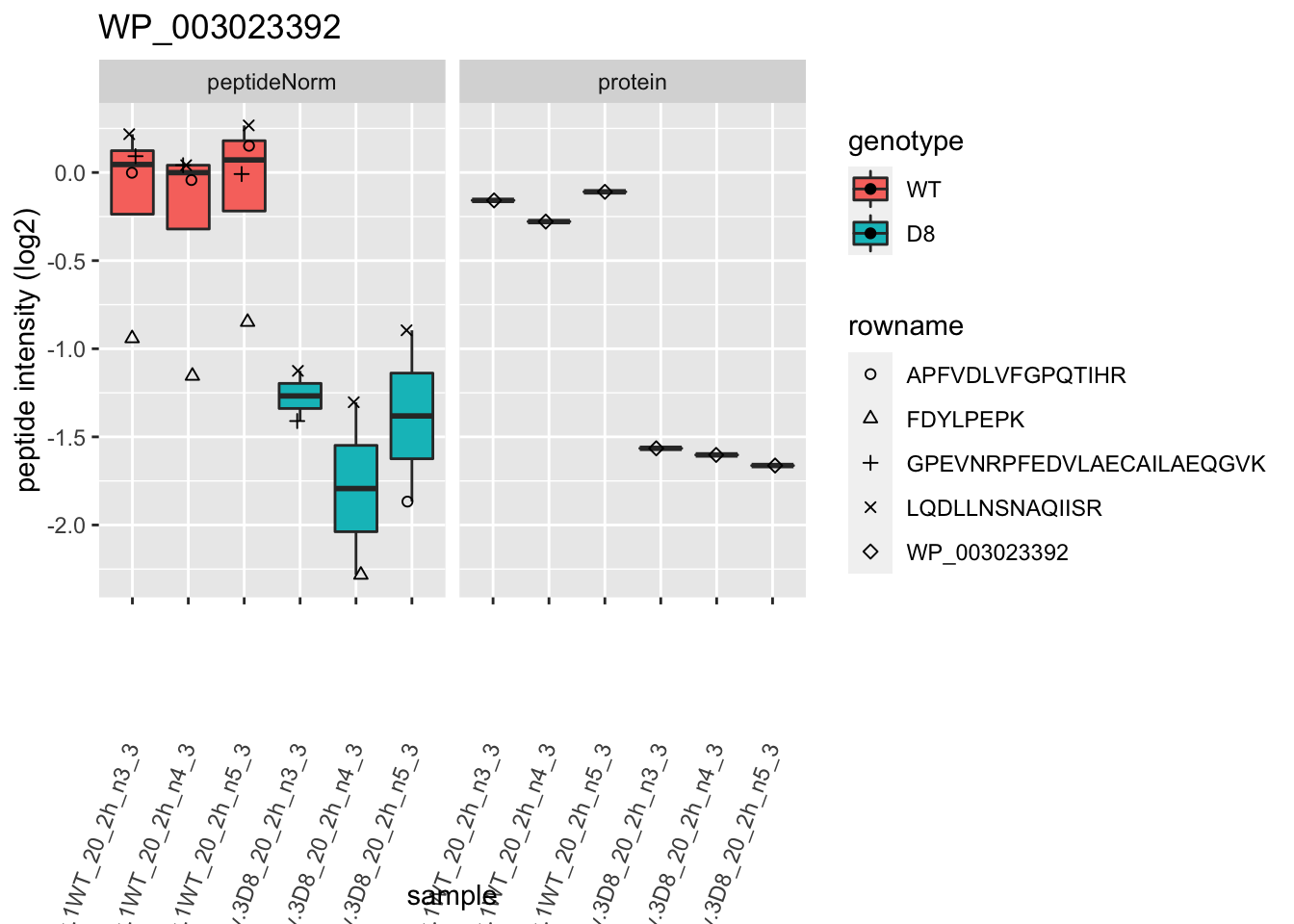
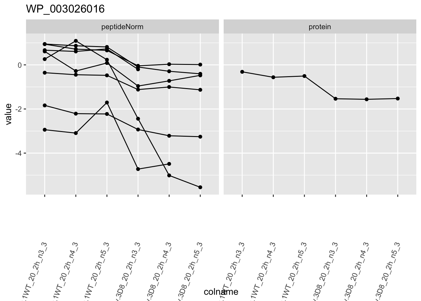
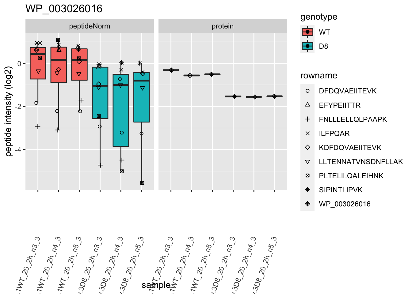
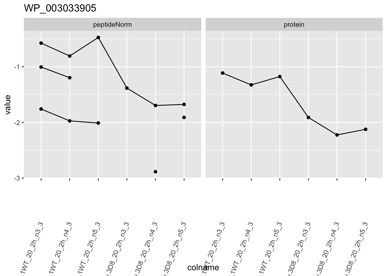
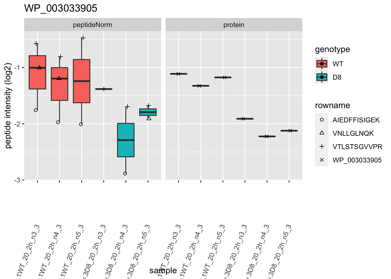
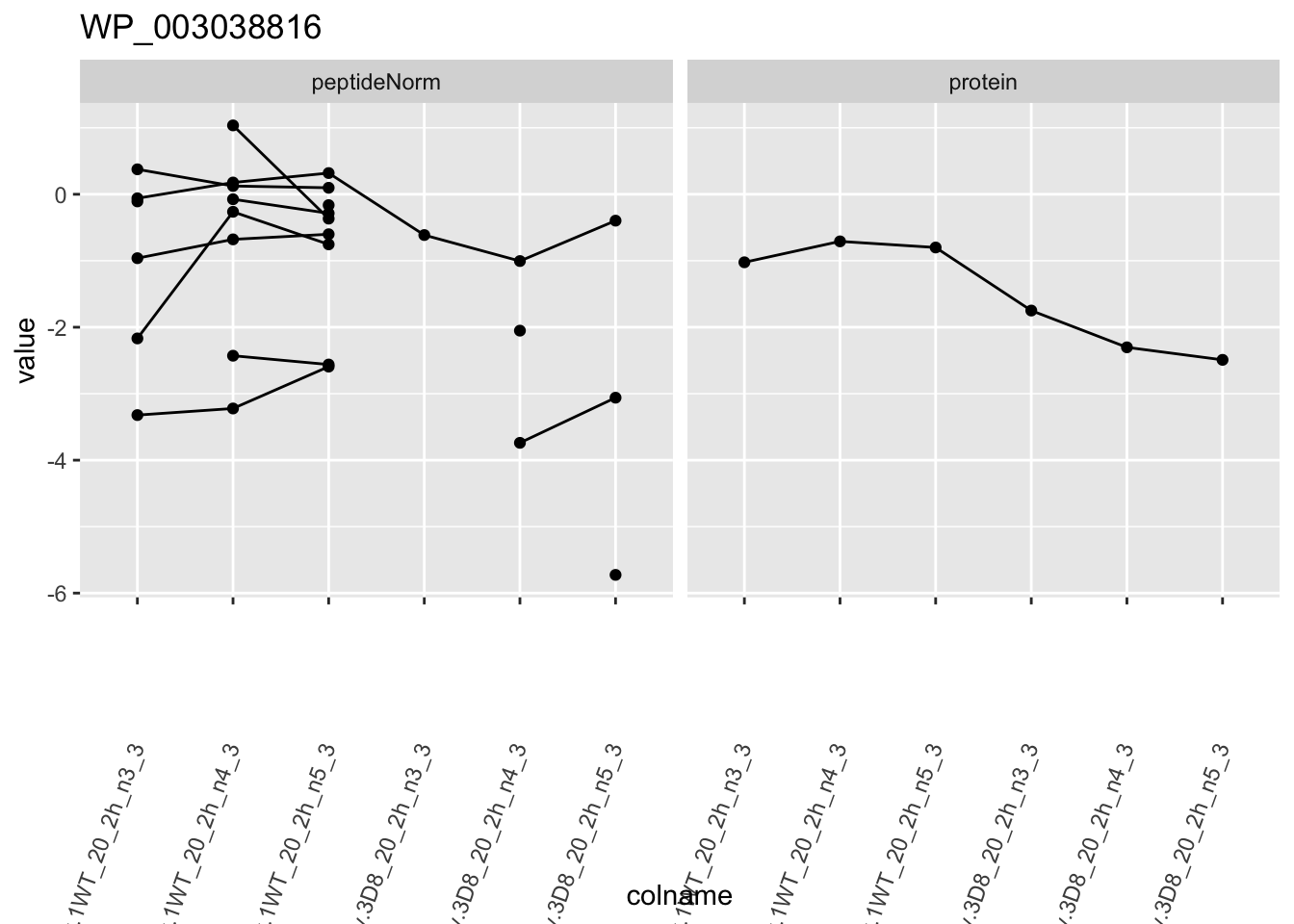
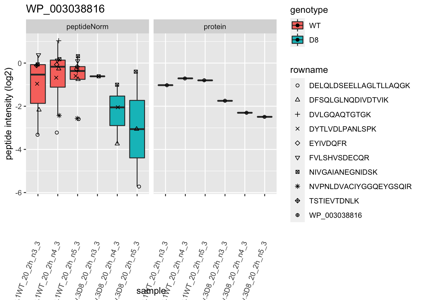
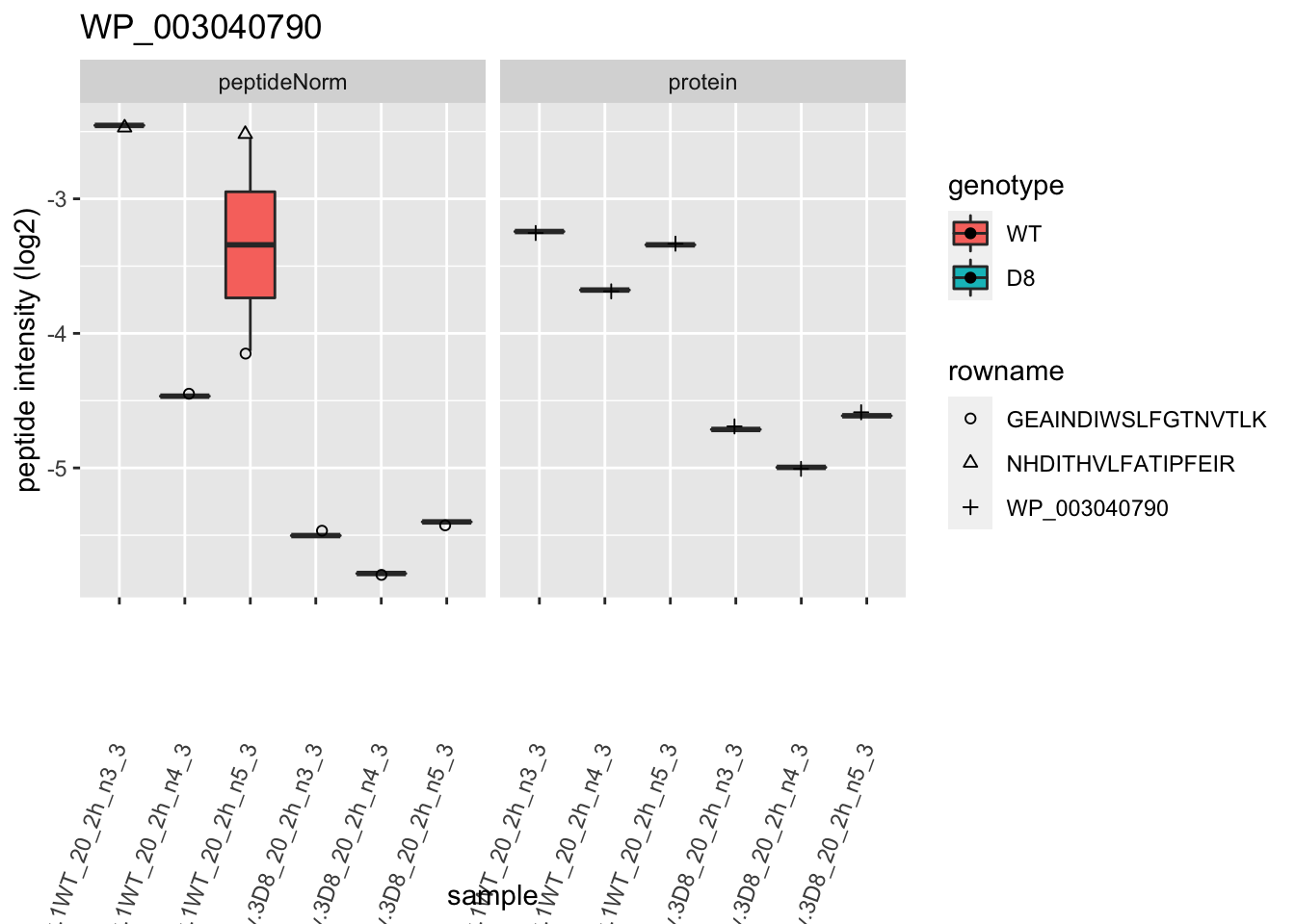
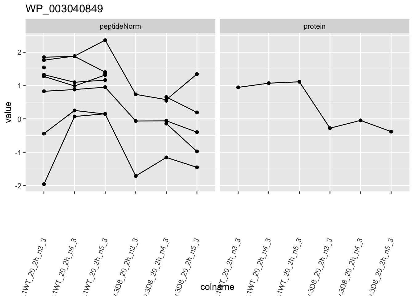
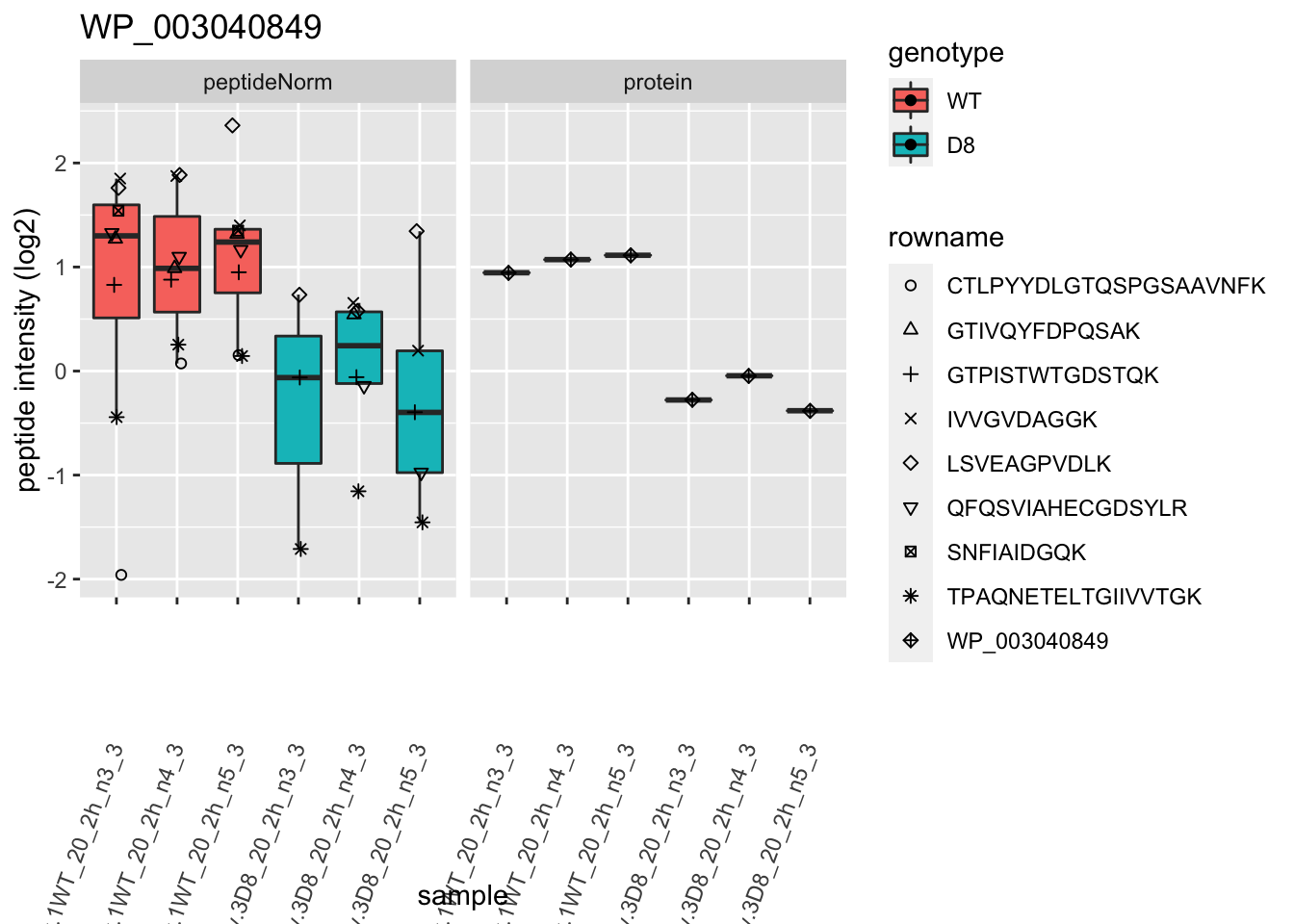
1.6 Plots

sigNames <- rowData(pe[["protein"]])$genotypeD8 %>%
    rownames_to_column("protein") %>%
    filter(adjPval < 0.05) %>%
    pull(protein)
heatmap(assay(pe[["protein"]])[sigNames, ])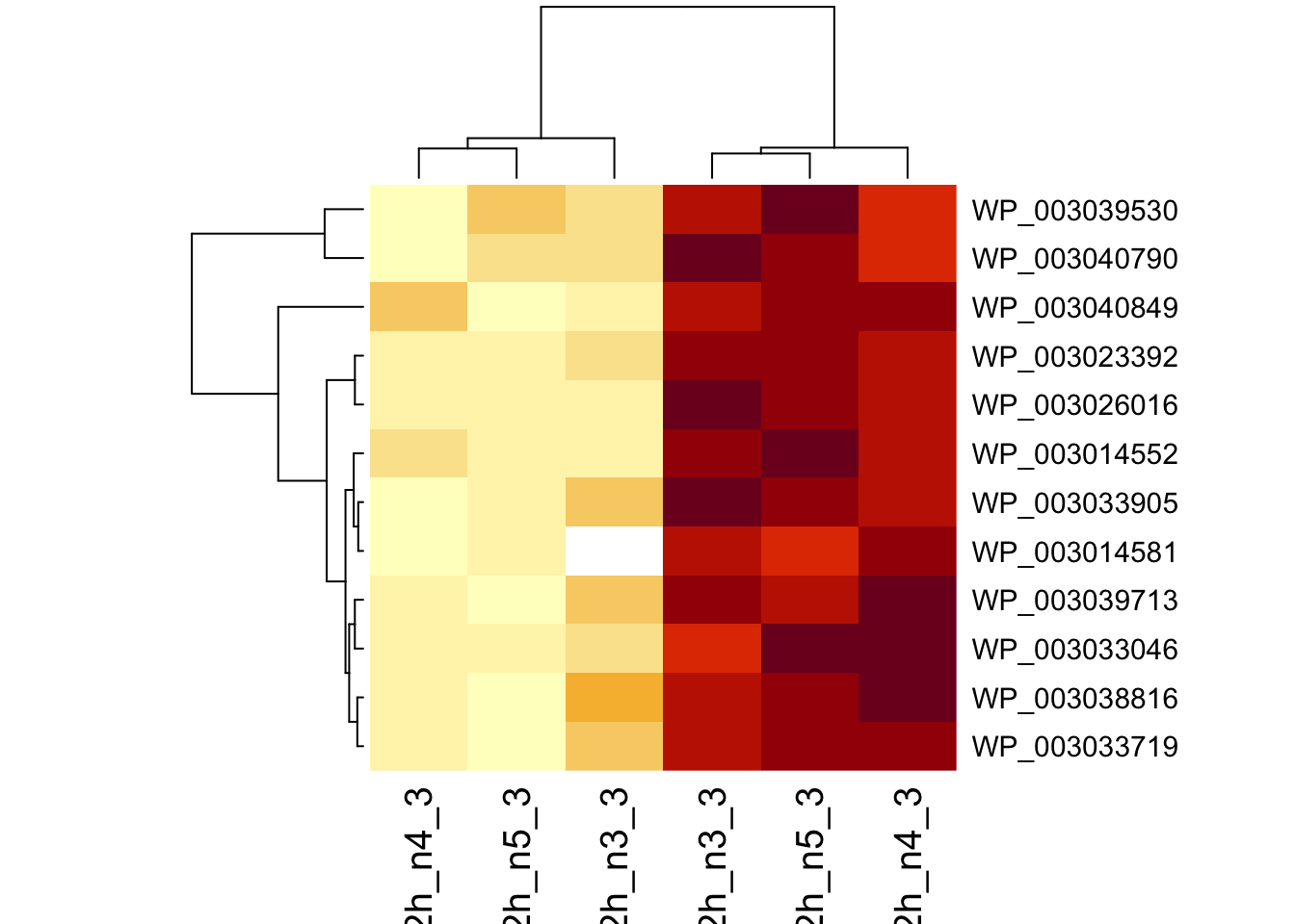

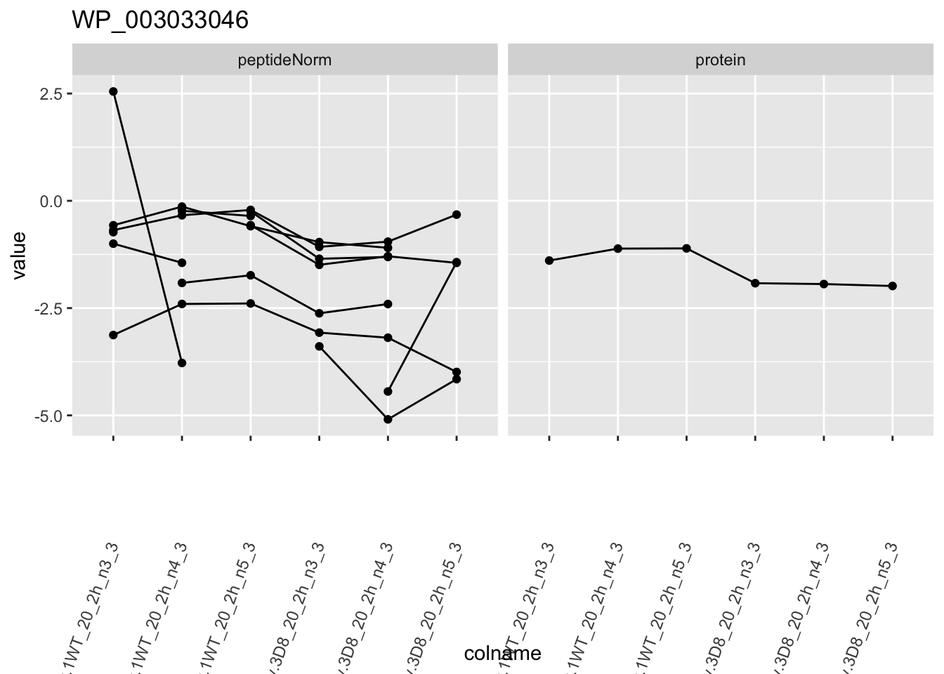
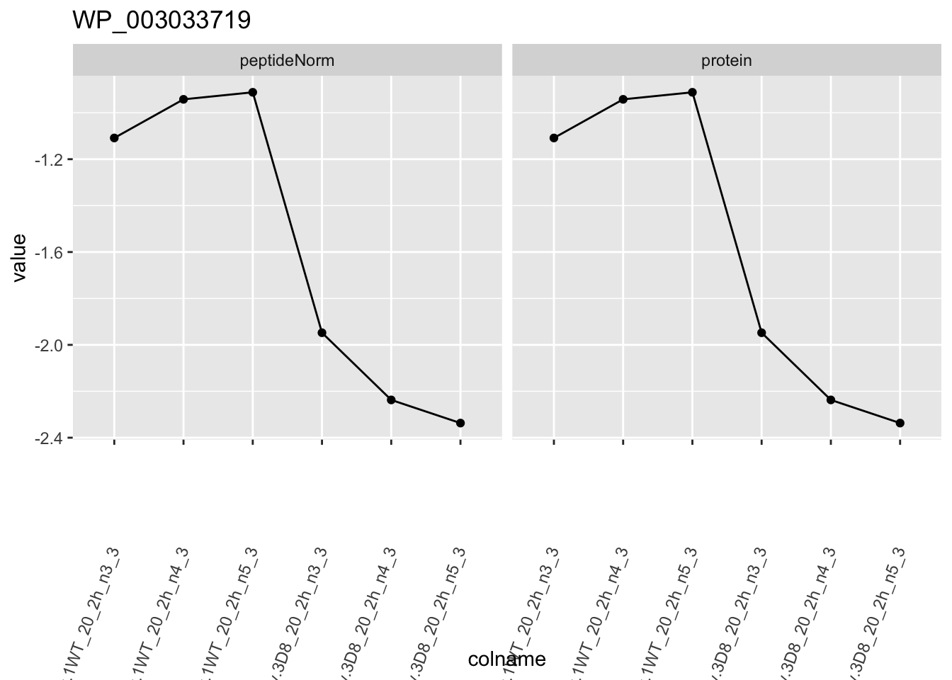
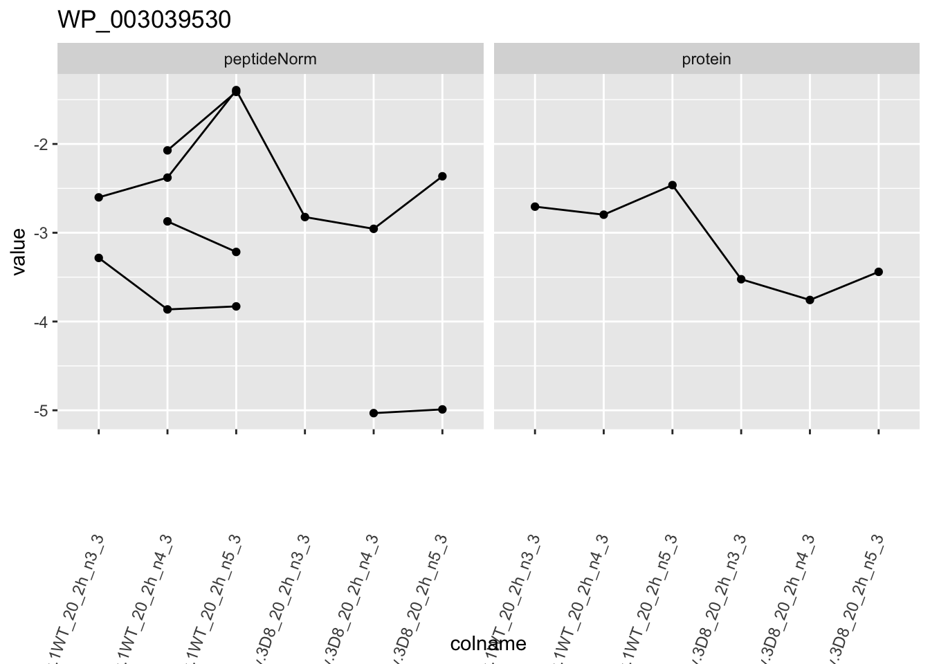
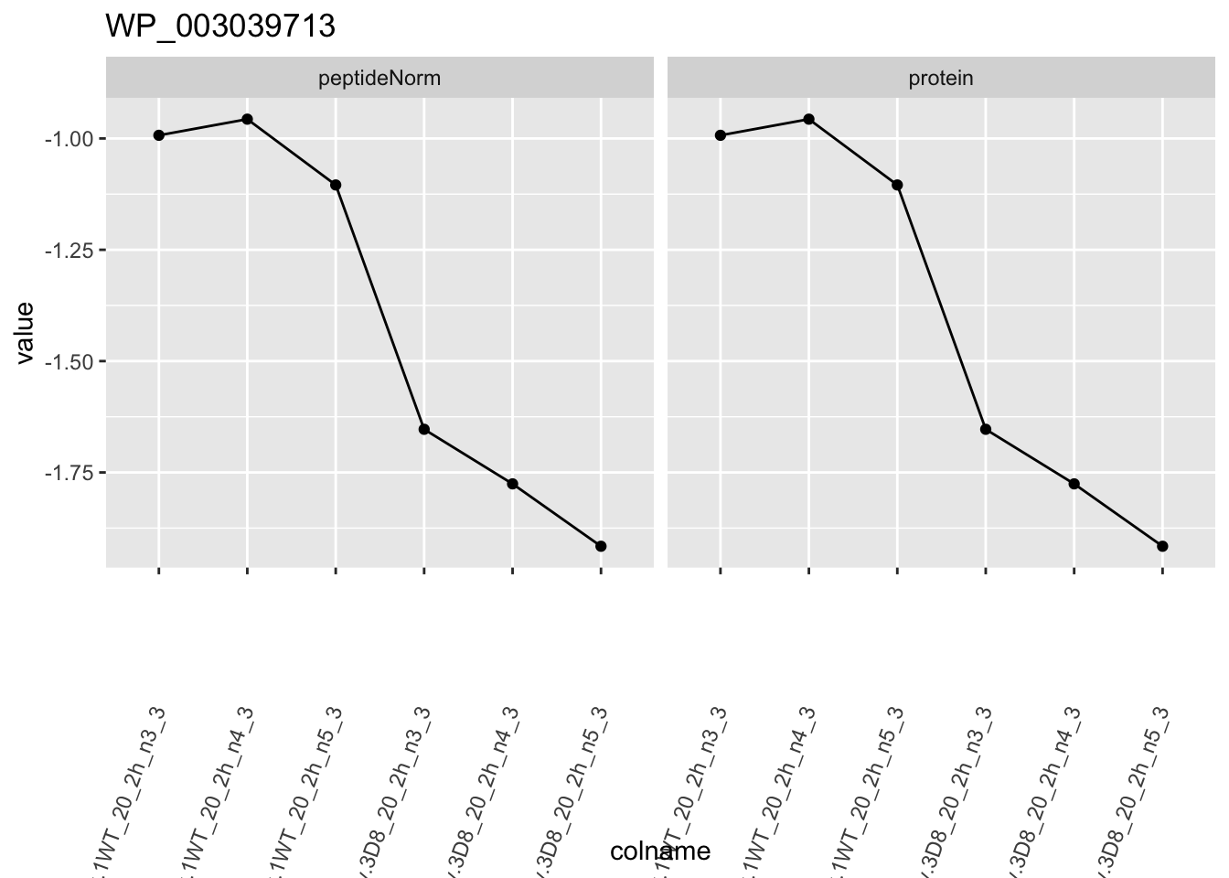
for (protName in sigNames)
    {
        pePlot <- pe[protName, , c("peptideNorm", "protein")]
        pePlotDf <- data.frame(longFormat(pePlot))
        pePlotDf$assay <- factor(pePlotDf$assay,
            levels = c("peptideNorm", "protein")
        )
        pePlotDf$genotype <- as.factor(colData(pePlot)[pePlotDf$colname, "genotype"])

        # plotting
        p1 <- ggplot(
            data = pePlotDf,
            aes(x = colname, y = value, group = rowname)
        ) +
            geom_line() +
            geom_point() +
            facet_grid(~assay) +
            theme(axis.text.x = element_text(angle = 70, hjust = 1, vjust = 0.5)) +
            ggtitle(protName)
        print(p1)

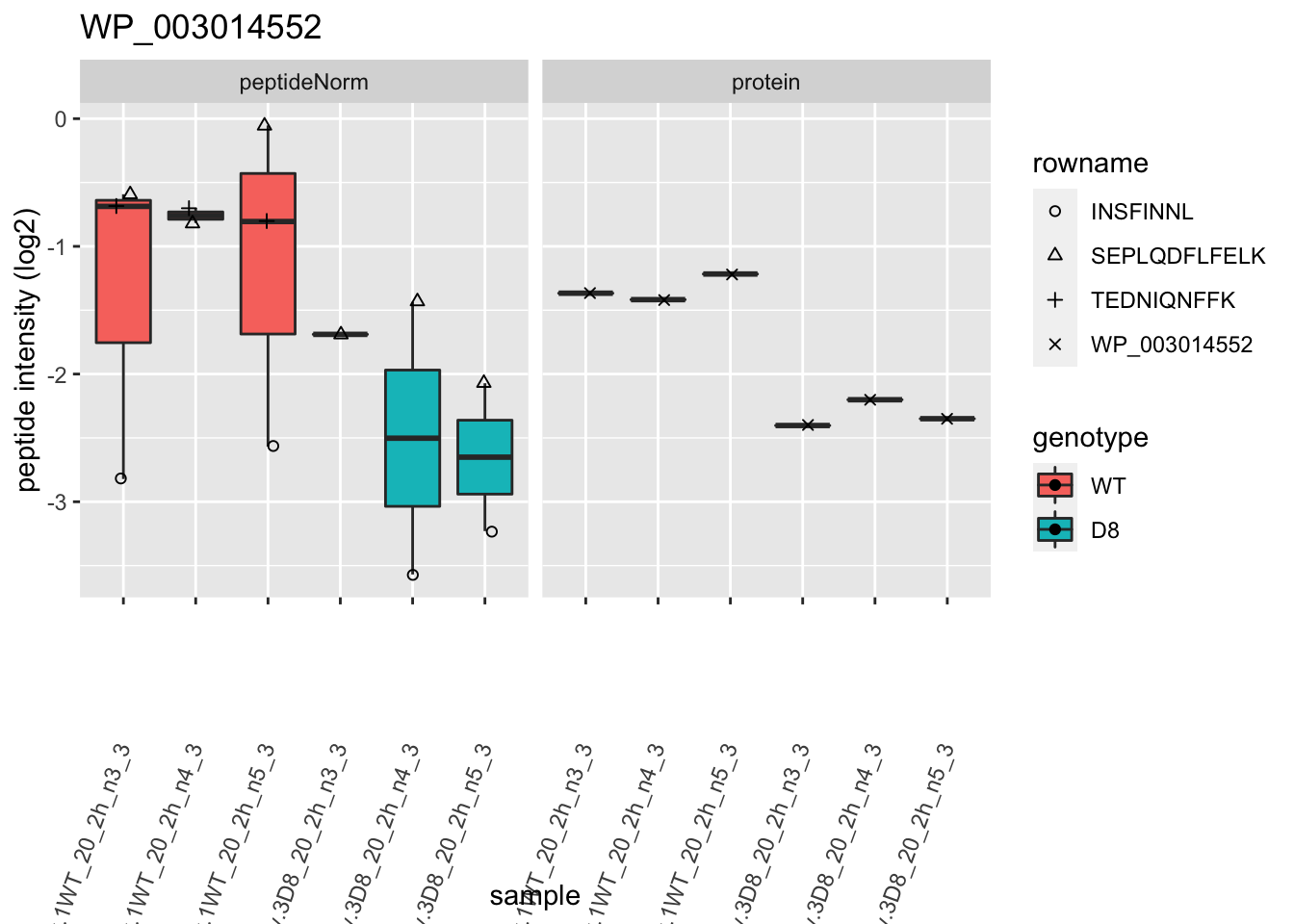
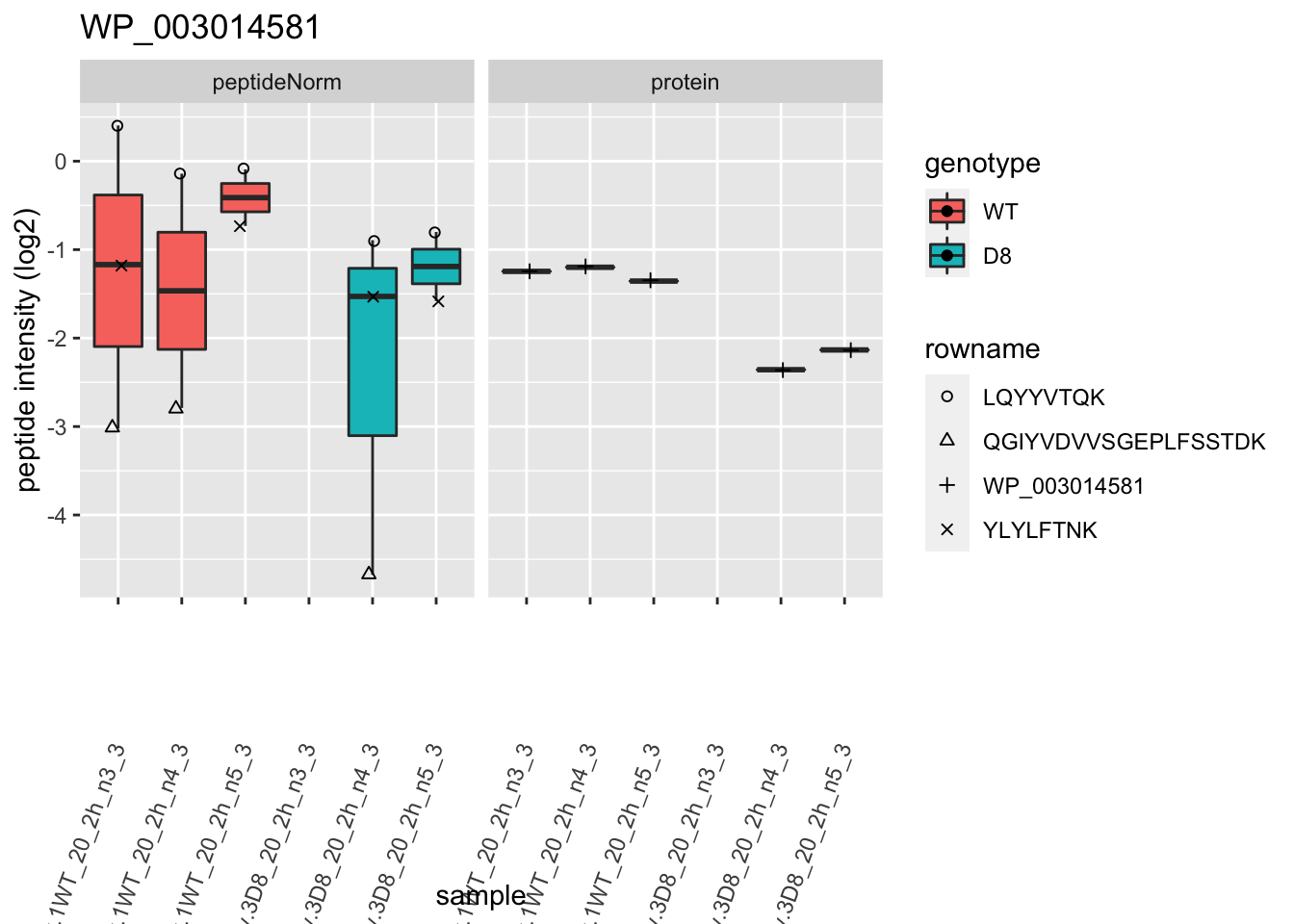
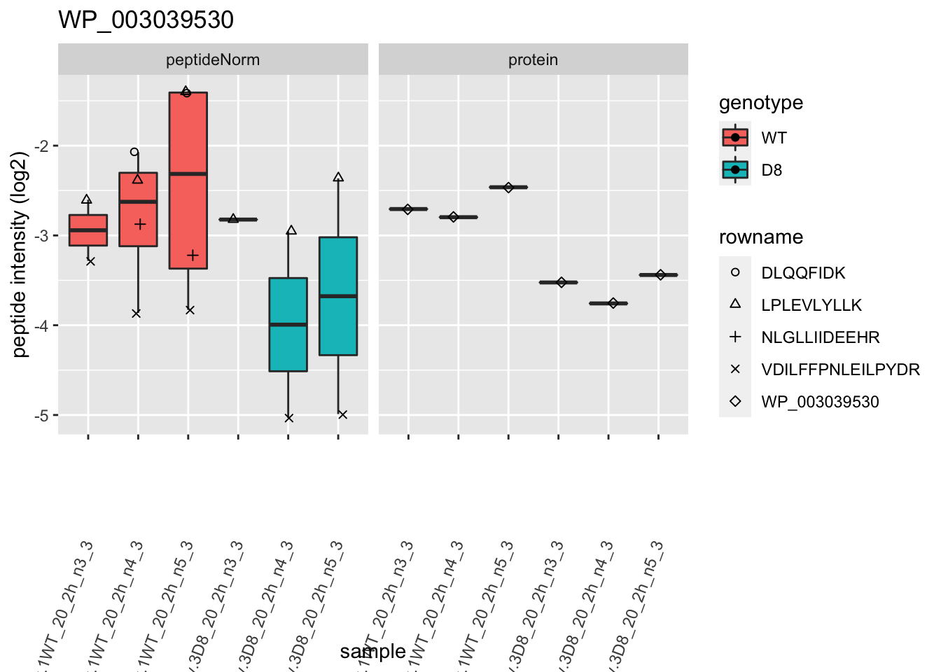
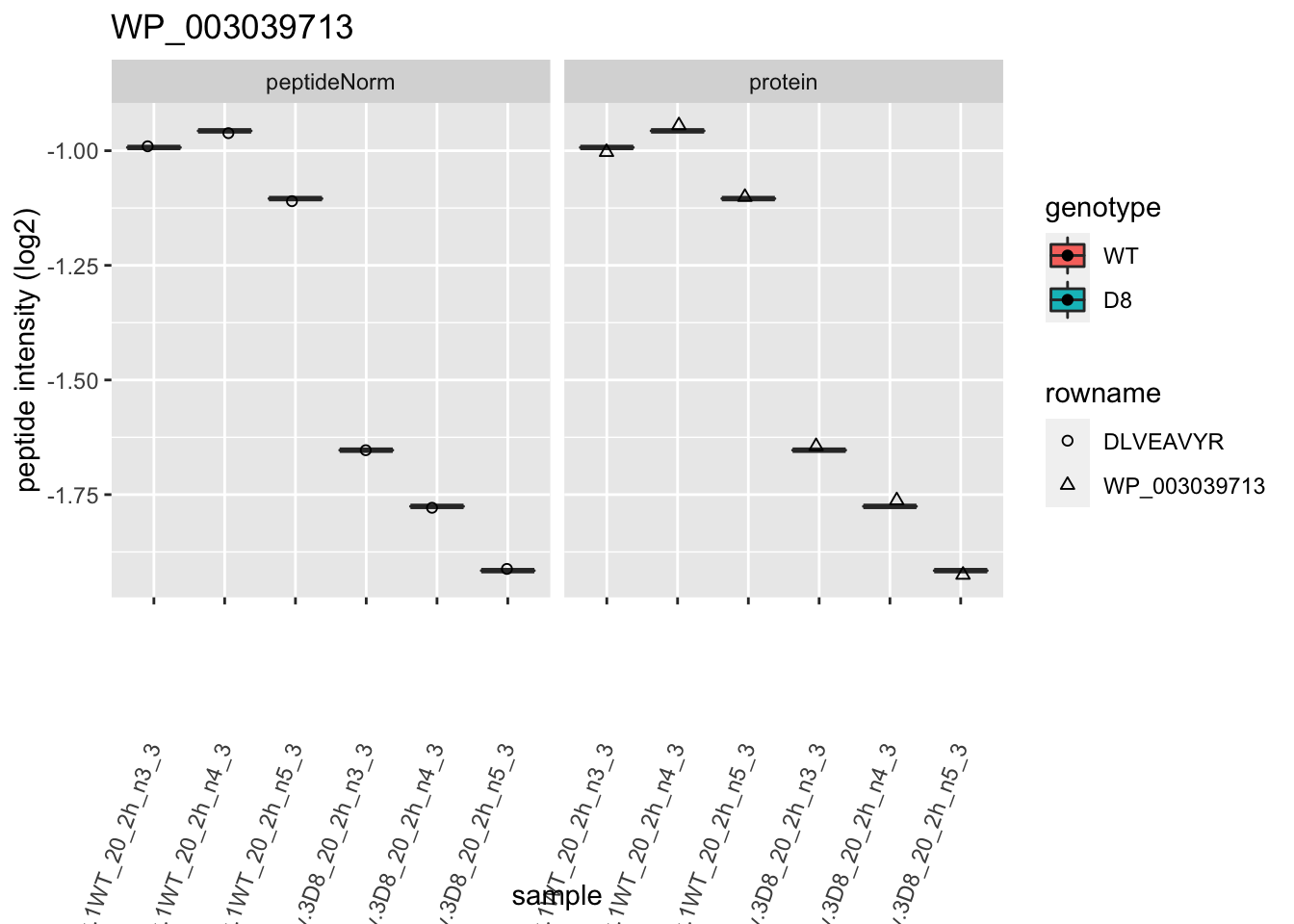
        # plotting 2
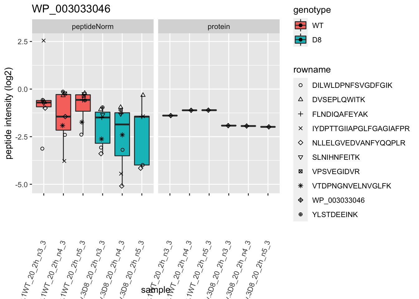
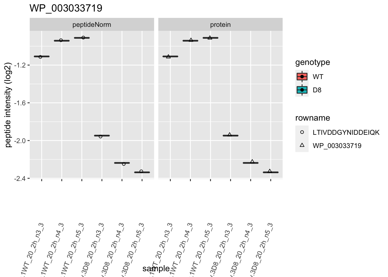
        p2 <- ggplot(pePlotDf, aes(x = colname, y = value, fill = genotype)) +
            geom_boxplot(outlier.shape = NA) +
            geom_point(
                position = position_jitter(width = .1),
                aes(shape = rowname)
            ) +
            scale_shape_manual(values = 1:nrow(pePlotDf)) +
            labs(title = protName, x = "sample", y = "peptide intensity (log2)") +
            theme(axis.text.x = element_text(angle = 70, hjust = 1, vjust = 0.5)) +
            facet_grid(~assay)
        print(p2)
}

2 Experimental Design

2.1 Sample size

\[ \log_2 \text{FC} = \bar{y}_{p1}-\bar{y}_{p2} \]

\[ T_g=\frac{\log_2 \text{FC}}{\text{se}_{\log_2 \text{FC}}} \]

\[ T_g=\frac{\widehat{\text{signal}}}{\widehat{\text{Noise}}} \]

If we can assume equal variance in both treatment groups:

\[ \text{se}_{\log_2 \text{FC}}=\text{SD}\sqrt{\frac{1}{n_1}+\frac{1}{n_2}} \]

\(\rightarrow\) if number of bio-repeats increases we have a higher power!

• cfr. Study of tamoxifen treated Estrogen Recepter (ER) positive breast cancer patients

2.2 Blocking

\[\sigma^2= \sigma^2_{bio}+\sigma^2_\text{lab} +\sigma^2_\text{extraction} + \sigma^2_\text{run} + \ldots\]

• Biological: fluctuations in protein level between mice, fluctations in protein level between cells, …
• Technical: cage effect, lab effect, week effect, plasma extraction, MS-run, …

2.3 Nature methods: Points of significance - Blocking

https://www.nature.com/articles/nmeth.3005.pdf

2.4 Mouse example

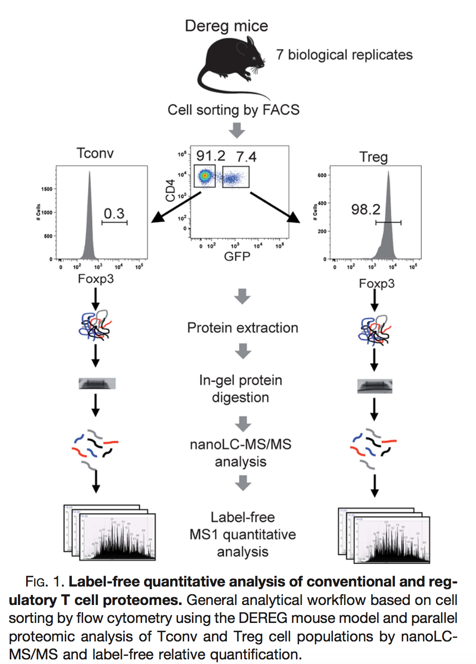Duguet et al. (2017) MCP 16(8):1416-1432. doi: 10.1074/mcp.m116.062745

• All treatments of interest are present within block!
• We can estimate the effect of the treatment within block!
• We can isolate the between block variability from the analysis using linear model: \[ y \sim \text{type} + \text{mouse} \]
• Not possible with Perseus!

2.4.1 Assess the impact of blocking in the tutorial session!

• Completely randomized design with only one cell type per mouse (Treg and Tconv)

\[\updownarrow\]

• Randomized complete block design assessing Treg and Tconv on each mouse

3 Software & code

• Our R/Bioconductor package msqrob2 can be used in R markdown scripts or with a GUI/shinyApp in the msqrob2gui package.

• The GUI is intended as a introduction to the key concepts of proteomics data analysis for users who have no experience in R.

• However, learning how to code data analyses in R markdown scripts is key for open en reproducible science and for reporting your proteomics data analyses and interpretation in a reproducible way.

• More information on our tools can be found in our papers (Goeminne, Gevaert, and Clement 2016), (Goeminne et al. 2020) and (Sticker et al. 2020). Please refer to our work when using our tools.

• Clips on the code on importing the data and preprocessing can be found in Part I Preprocessing

• A clip on the code for modelling and statistical inference with msqrob2 is included below

References

Goeminne, L. J. E., A. Sticker, L. Martens, K. Gevaert, and L. Clement. 2020. “MSqRob Takes the Missing Hurdle: Uniting Intensity- and Count-Based Proteomics.” Anal Chem 92 (9): 6278–87.

Goeminne, L. J., K. Gevaert, and L. Clement. 2016. “Peptide-level Robust Ridge Regression Improves Estimation, Sensitivity, and Specificity in Data-dependent Quantitative Label-free Shotgun Proteomics.” Mol Cell Proteomics 15 (2): 657–68.

Sticker, A., L. Goeminne, L. Martens, and L. Clement. 2020. “Robust Summarization and Inference in Proteome-wide Label-free Quantification.” Mol Cell Proteomics 19 (7): 1209–19.