Sources of variability in label-free proteomics experiments

This is part of the online course Experimental Design and Data-Analysis in Label-Free Quantitative LC/MS Proteomics - A Tutorial with msqrob2 (hupo21)

Click to see libraries that are loaded

library(tidyverse)
library(limma)
library(QFeatures)
library(msqrob2)
library(plotly)
library(gridExtra)

1 Intro

1. Background + cptac study
2. Sources of variability
3. Summarization

1.1 MS-based workflow

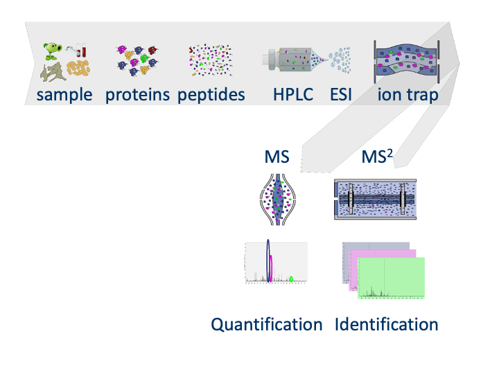
• Peptide Characteristics

  • Modifications
  • Ionisation Efficiency: huge variability
  • Identification
    • Misidentification \(\rightarrow\) outliers
    • MS\(^2\) selection on peptide abundance
    • Context depending missingness
    • Non-random missingness

\(\rightarrow\) Unbalanced pepide identifications across samples and messy data

1.2 CPTAC Spike-in Study

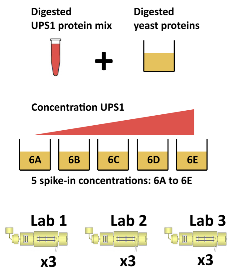
• Same trypsin-digested yeast proteome background in each sample

• Trypsin-digested Sigma UPS1 standard: 48 different human proteins spiked in at 5 different concentrations (treatment A-E)

• Samples repeatedly run on different instruments in different labs

• After MaxQuant search with match between runs option

  • 41% of all proteins are quantified in all samples
  • 6.6% of all peptides are quantified in all samples

\(\rightarrow\) vast amount of missingness

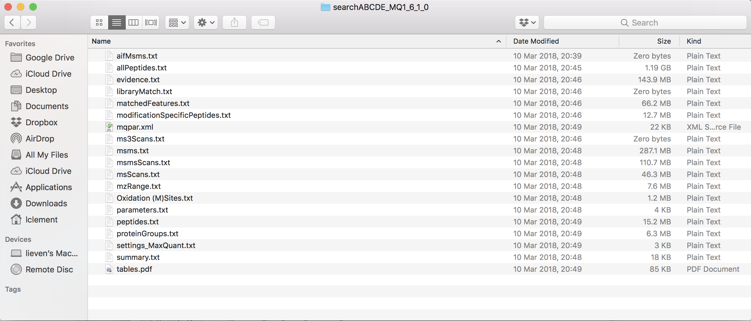
1.2.1 Maxquant output

1.2.2 Read data

Click to see background and code

1. We use a peptides.txt file from MS-data quantified with maxquant that contains MS1 intensities summarized at the peptide level.

peptidesFile <- "https://raw.githubusercontent.com/statOmics/PDA21/data/quantification/fullCptacDatasSetNotForTutorial/peptides.txt"

2. Maxquant stores the intensity data for the different samples in columnns that start with Intensity. We can retreive the column names with the intensity data with the code below:

ecols <- grep("Intensity\\.", names(read.delim(peptidesFile)))

3. Read the data and store it in QFeatures object

pe <- readQFeatures(
  table = peptidesFile,
  fnames = 1,
  ecol = ecols,
  name = "peptideRaw", sep="\t")

1.2.3 Design

Click to see background and code

pe %>% colnames

## CharacterList of length 1
## [["peptideRaw"]] Intensity.6A_1 Intensity.6A_2 ... Intensity.6E_9

• Note, that the sample names include the spike-in condition.

• They also end on a number.

  • 1-3 is from lab 1,
  • 4-6 from lab 2 and
  • 7-9 from lab 3.

• We update the colData with information on the design

colData(pe)$lab <- rep(rep(paste0("lab",1:3),each=3),5) %>% as.factor
colData(pe)$condition <- pe[["peptideRaw"]] %>% colnames %>% substr(12,12) %>% as.factor
colData(pe)$spikeConcentration <- rep(c(A = 0.25, B = 0.74, C = 2.22, D = 6.67, E = 20),each = 9)

• We explore the colData

colData(pe)

## DataFrame with 45 rows and 3 columns
##                     lab condition spikeConcentration
##                <factor>  <factor>          <numeric>
## Intensity.6A_1     lab1         A               0.25
## Intensity.6A_2     lab1         A               0.25
## Intensity.6A_3     lab1         A               0.25
## Intensity.6A_4     lab2         A               0.25
## Intensity.6A_5     lab2         A               0.25
## ...                 ...       ...                ...
## Intensity.6E_5     lab2         E                 20
## Intensity.6E_6     lab2         E                 20
## Intensity.6E_7     lab3         E                 20
## Intensity.6E_8     lab3         E                 20
## Intensity.6E_9     lab3         E                 20

2 Sources of variation

2.1 Intensities of one peptide

Peptide AALEELVK from spiked-in UPS protein P12081. We only show data from lab1.

Click to see code to make plot

subset <- pe["AALEELVK",colData(pe)$lab=="lab1"]
plotWhyLog <- data.frame(concentration = colData(subset)$spikeConcentration,
           y = assay(subset[["peptideRaw"]]) %>% c
           ) %>% 
  ggplot(aes(concentration, y)) +
  geom_point() +
  xlab("concentration (fmol/l)") +
  ggtitle("peptide AALEELVK in lab1")

plotWhyLog

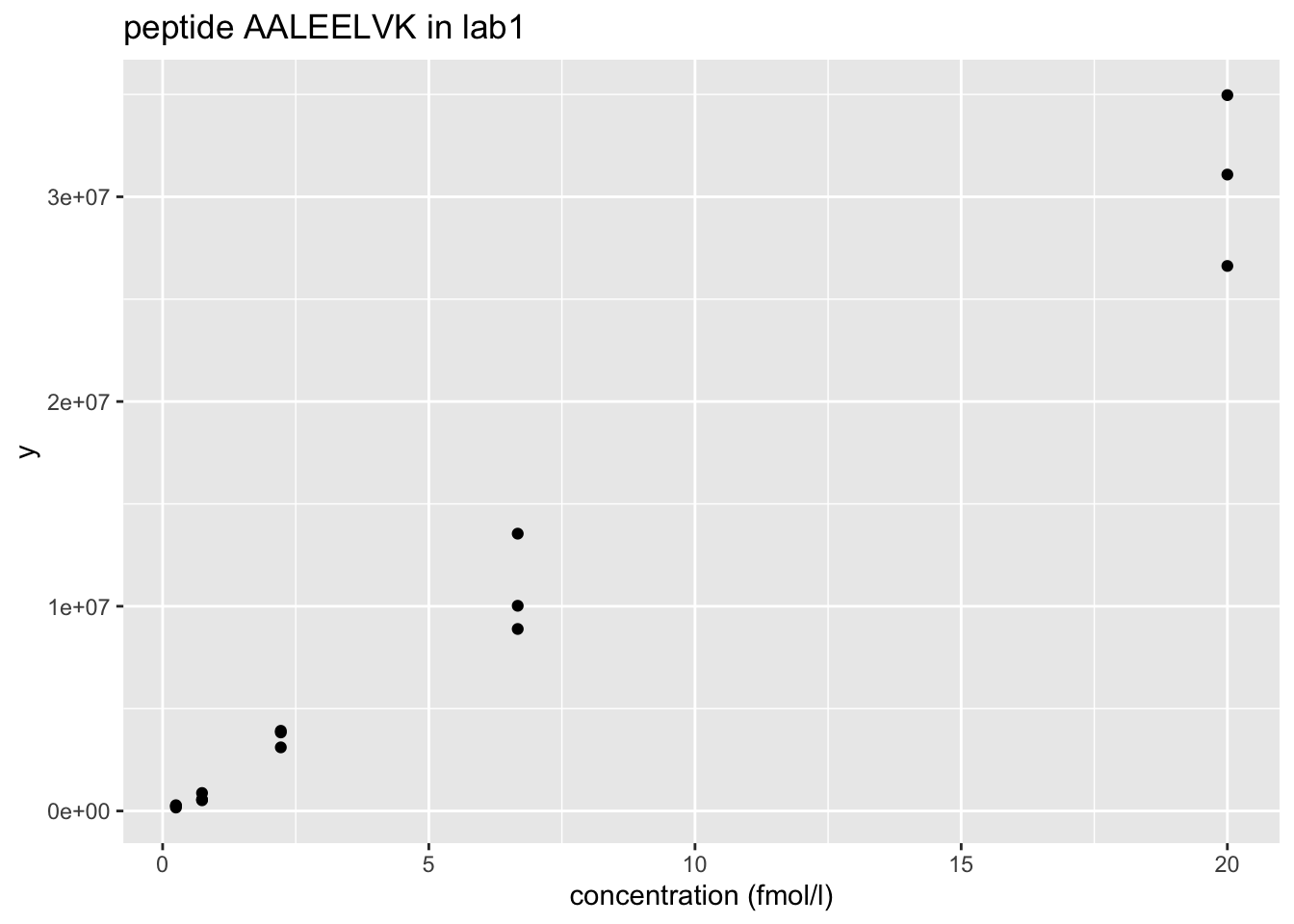
• Variance increases with the mean \(\rightarrow\) Multiplicative error structure

Click to see code to make plot

plotLog <- data.frame(concentration = colData(subset)$spikeConcentration,
           y = assay(subset[["peptideRaw"]]) %>% c
           ) %>% 
  ggplot(aes(concentration, y)) +
  geom_point() + 
  scale_x_continuous(trans='log2') + 
  scale_y_continuous(trans='log2') +
  xlab("concentration (fmol/l)") +
  ggtitle("peptide AALEELVK in lab1 with axes on log scale")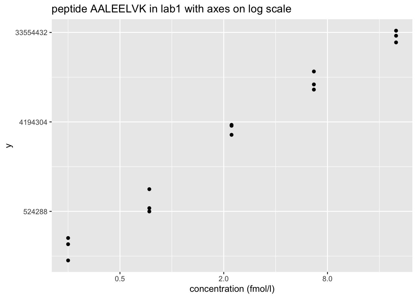

plotLog

• Data seems to be homoscedastic on log-scale \(\rightarrow\) log transformation of the intensity data
• In quantitative proteomics analysis on \(\log_2\)

\(\rightarrow\) Differences on a \(\log_2\) scale: \(\log_2\) fold changes

\[ \log_2 B - \log_2 A = \log_2 \frac{B}{A} = \log FC_\text{B - A} \] \[ \begin{array} {l} log_2 FC = 1 \rightarrow FC = 2^1 =2\\ log_2 FC = 2 \rightarrow FC = 2^2 = 4\\ \end{array} \]

2.2 Log-transform

Click to see code to log-transfrom the data

• We calculate how many non zero intensities we have for each peptide and this can be useful for filtering.

rowData(pe[["peptideRaw"]])$nNonZero <- rowSums(assay(pe[["peptideRaw"]]) > 0)

• Peptides with zero intensities are missing peptides and should be represent with a NA value rather than 0.

pe <- zeroIsNA(pe, "peptideRaw") # convert 0 to NA

• Logtransform data with base 2

pe <- logTransform(pe, base = 2, i = "peptideRaw", name = "peptideLog")

2.3 Filtering

Click to see code to filter the data

1. Handling overlapping protein groups

In our approach a peptide can map to multiple proteins, as long as there is none of these proteins present in a smaller subgroup.

pe <- filterFeatures(pe, ~ Proteins %in% smallestUniqueGroups(rowData(pe[["peptideLog"]])$Proteins))

2. Remove reverse sequences (decoys) and contaminants

We now remove the contaminants, peptides that map to decoy sequences, and proteins which were only identified by peptides with modifications.

pe <- filterFeatures(pe,~Reverse != "+")
pe <- filterFeatures(pe,~ Potential.contaminant != "+")

3. Drop peptides that were only identified in one sample

We keep peptides that were observed at last twice.

pe <- filterFeatures(pe,~ nNonZero >=2)
nrow(pe[["peptideLog"]])

## [1] 10478

We keep 10478 peptides upon filtering.

2.4 Technical Variability

Click to see code for plot

densityConditionD <- pe[["peptideLog"]][,colData(pe)$condition=="D"] %>% 
  assay %>%
  as.data.frame() %>%
  gather(sample, intensity) %>% 
  mutate(lab = colData(pe)[sample,"lab"]) %>%
  ggplot(aes(x=intensity,group=sample,color=lab)) + 
    geom_density() +
    ggtitle("condition D")

densityLab2 <- pe[["peptideLog"]][,colData(pe)$lab=="lab2"] %>% 
  assay %>%
  as.data.frame() %>%
  gather(sample, intensity) %>% 
  mutate(condition = colData(pe)[sample,"condition"]) %>%
  ggplot(aes(x=intensity,group=sample,color=condition)) + 
    geom_density() +
    ggtitle("lab2")

densityConditionD

## Warning: Removed 39179 rows containing non-finite values (stat_density).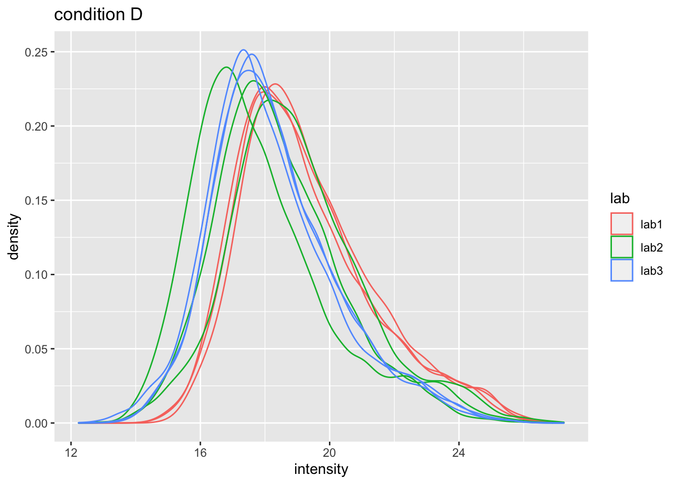

densityLab2

## Warning: Removed 44480 rows containing non-finite values (stat_density).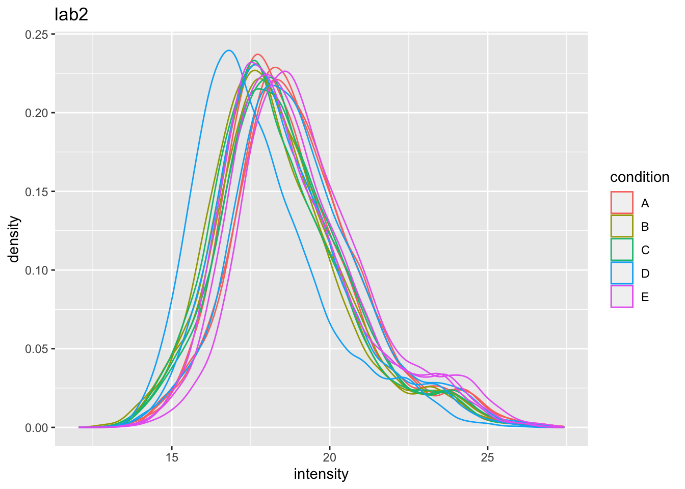

• Even in very clean synthetic dataset (same background, only 48 UPS proteins can be different) the marginal peptide intensity distribution across samples can be quite distinct

• Considerable effects between and within labs for replicate samples

• Considerable effects between samples with different spike-in concentration

\(\rightarrow\) Normalization is needed

---

2.5 Normalization

Normalization of the data by median centering

\[y_{ip}^\text{norm} = y_{ip} - \hat\mu_i\] with \(\hat\mu_i\) the median intensity over all observed peptides in sample \(i\).

Click to see R-code to normalize the data

pe <- normalize(pe, 
                i = "peptideLog", 
                name = "peptideNorm", 
                method = "center.median")

Click to see code to make plot

densityConditionDNorm <- pe[["peptideNorm"]][,colData(pe)$condition=="D"] %>% 
  assay %>%
  as.data.frame() %>%
  gather(sample, intensity) %>% 
  mutate(lab = colData(pe)[sample,"lab"]) %>%
  ggplot(aes(x=intensity,group=sample,color=lab)) + 
    geom_density() +
    ggtitle("condition D")

densityLab2Norm <- pe[["peptideNorm"]][,colData(pe)$lab=="lab2"] %>% 
  assay %>%
  as.data.frame() %>%
  gather(sample, intensity) %>% 
  mutate(condition = colData(pe)[sample,"condition"]) %>%
  ggplot(aes(x=intensity,group=sample,color=condition)) + 
    geom_density() +
    ggtitle("lab2")

densityConditionDNorm

## Warning: Removed 39179 rows containing non-finite values (stat_density).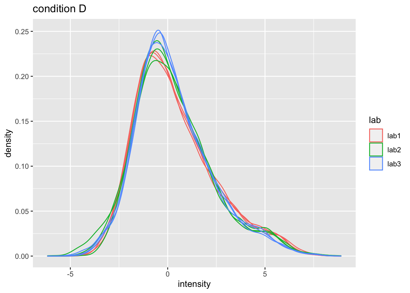

densityLab2Norm

## Warning: Removed 44480 rows containing non-finite values (stat_density).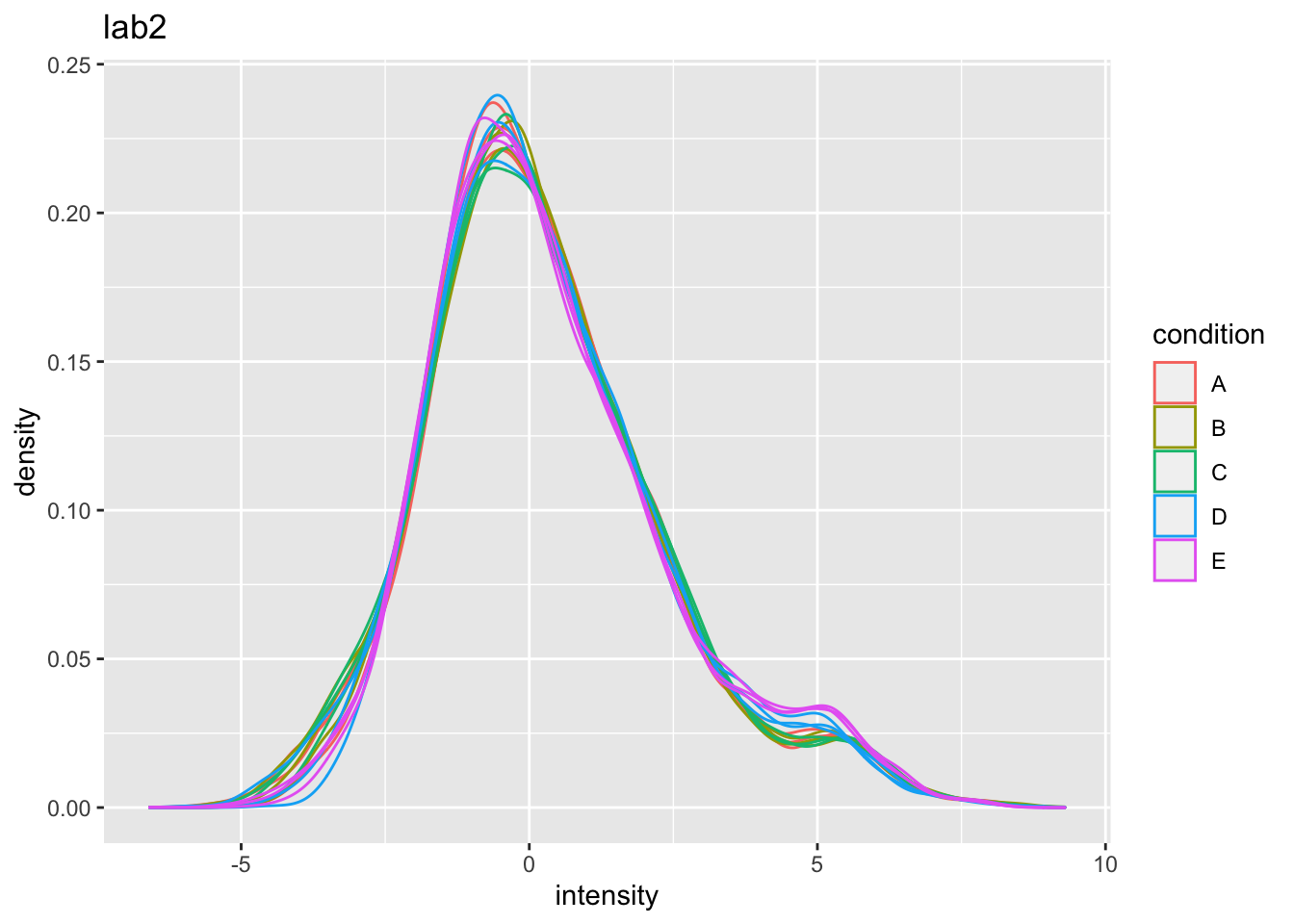

2.6 Pseudo replication

Click to see code to make plot

prot <- "P01031ups|CO5_HUMAN_UPS"
data <- pe[["peptideNorm"]][
  rowData(pe[["peptideNorm"]])$Proteins == prot,
  colData(pe)$lab=="lab3"] %>%
  assay %>%
  as.data.frame %>%
  rownames_to_column(var = "peptide") %>%
  gather(sample, intensity, -peptide) %>% 
  mutate(condition = colData(pe)[sample,"condition"]) %>%
  na.exclude
sumPlot <- data %>%
  ggplot(aes(x = peptide, y = intensity, color = condition, group = sample, label = condition), show.legend = FALSE) +
  geom_text(show.legend = FALSE) +
  theme_minimal() +
  theme(axis.text.x = element_text(angle = 90, vjust = 0.5, hjust = 1)) +
  xlab("Peptide") + 
  ylab("Intensity (log2)") +
  ggtitle(paste0("protein: ",prot))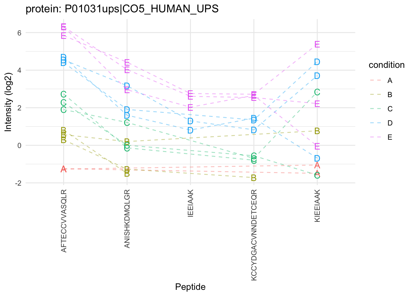

sumPlot +
  geom_line(linetype="dashed",alpha=.4)

• Sources of variability in plot:

  • Between treatment variability
  • Between sample variability
  • Between peptide variability
  • within sample variability

• Multiple peptides from same protein in a sample

• Peptide intensities in the same sample are correlated: Pseudo replication

\(\rightarrow\) Summarization!

• Strong peptide effect
• Unbalanced peptide identification

2.6.1 Illustration on subset of CPTAC study: A vs B comparison in lab 3

2.6.1.1 LFQ

Click to see background and code

1. Import data

proteinsFile <- "https://raw.githubusercontent.com/statOmics/PDA21/data/quantification/cptacAvsB_lab3/proteinGroups.txt"

ecols <- grep("LFQ\\.intensity\\.", names(read.delim(proteinsFile)))

peLFQ <- readQFeatures(
  table = proteinsFile, fnames = 1, ecol = ecols,
  name = "proteinRaw", sep = "\t"
)

cond <- which(
  strsplit(colnames(peLFQ)[[1]][1], split = "")[[1]] == "A") # find where condition is stored

colData(peLFQ)$condition <- substr(colnames(peLFQ), cond, cond) %>%
  unlist %>%  
  as.factor

2. Preprocessing

rowData(peLFQ[["proteinRaw"]])$nNonZero <- rowSums(assay(peLFQ[["proteinRaw"]]) > 0)

peLFQ <- zeroIsNA(peLFQ, "proteinRaw") # convert 0 to NA

peLFQ <- logTransform(peLFQ, base = 2, i = "proteinRaw", name = "proteinLog")

peLFQ <- filterFeatures(peLFQ,~ Reverse != "+")
peLFQ <- filterFeatures(peLFQ,~ Potential.contaminant != "+")

peLFQ <- normalize(peLFQ, 
                i = "proteinLog", 
                name = "protein", 
                method = "center.median")

3. Modeling and Inference

peLFQ <- msqrob(object = peLFQ, i = "protein", formula = ~condition)

L <- makeContrast("conditionB=0", parameterNames = c("conditionB"))
peLFQ <- hypothesisTest(object = peLFQ, i = "protein", contrast = L)

volcanoLFQ <- ggplot(rowData(peLFQ[["protein"]])$conditionB,
                  aes(x = logFC, y = -log10(pval), color = adjPval < 0.05)) +
  geom_point(cex = 2.5) +
  scale_color_manual(values = alpha(c("black", "red"), 0.5)) + 
  theme_minimal() +
  ggtitle(paste0("maxLFQ: TP = ",sum(rowData(peLFQ[["protein"]])$conditionB$adjPval<0.05&grepl(rownames(rowData(peLFQ[["protein"]])$conditionB),pattern ="UPS"),na.rm=TRUE), " FP = ", sum(rowData(peLFQ[["protein"]])$conditionB$adjPval<0.05&!grepl(rownames(rowData(peLFQ[["protein"]])$conditionB),pattern ="UPS"),na.rm=TRUE)))

2.6.1.2 Median & robust summarization

Click to see background and code

1. Import Data

peptidesFile <- "https://raw.githubusercontent.com/statOmics/SGA2020/data/quantification/cptacAvsB_lab3/peptides.txt"

ecols <- grep(
  "Intensity\\.", 
  names(read.delim(peptidesFile))
  )

peAB <- readQFeatures(
  table = peptidesFile,
  fnames = 1,
  ecol = ecols,
  name = "peptideRaw", sep="\t")

cond <- which(
  strsplit(colnames(peAB)[[1]][1], split = "")[[1]] == "A") # find where condition is stored

colData(peAB)$condition <- substr(colnames(peAB), cond, cond) %>%
  unlist %>%  
  as.factor

2. Preprocessing

rowData(peAB[["peptideRaw"]])$nNonZero <- rowSums(assay(peAB[["peptideRaw"]]) > 0)

peAB <- zeroIsNA(peAB, "peptideRaw") # convert 0 to NA

peAB <- logTransform(peAB, base = 2, i = "peptideRaw", name = "peptideLog")

peAB <- filterFeatures(peAB, ~ Proteins %in% smallestUniqueGroups(rowData(peAB[["peptideLog"]])$Proteins))

peAB <- filterFeatures(peAB,~Reverse != "+")
peAB <- filterFeatures(peAB,~ Potential.contaminant != "+")


peAB <- filterFeatures(peAB,~ nNonZero >=2)
nrow(peAB[["peptideLog"]])

## [1] 7011

peAB <- normalize(peAB, 
                i = "peptideLog", 
                name = "peptideNorm", 
                method = "center.median")

peAB <- aggregateFeatures(peAB,
  i = "peptideNorm",
  fcol = "Proteins",
  na.rm = TRUE,
  name = "proteinMedian",
  fun = matrixStats::colMedians)

peAB <- aggregateFeatures(peAB,
  i = "peptideNorm",
  fcol = "Proteins",
  na.rm = TRUE,
  name = "proteinRobust")

3. Modeling and inference

peAB <- msqrob(object = peAB, i = "proteinMedian", formula = ~condition)
L <- makeContrast("conditionB=0", parameterNames = c("conditionB"))
peAB <- hypothesisTest(object = peAB, i = "proteinMedian", contrast = L)

peAB <- msqrob(object = peAB, i = "proteinRobust", formula = ~condition)
peAB <- hypothesisTest(object = peAB, i = "proteinRobust", contrast = L)

volcanoMedian <- ggplot(rowData(peAB[["proteinMedian"]])$conditionB,
                  aes(x = logFC, y = -log10(pval), color = adjPval < 0.05)) +
  geom_point(cex = 2.5) +
  scale_color_manual(values = alpha(c("black", "red"), 0.5)) + 
  theme_minimal() +
  ggtitle(paste0("Median: TP = ",sum(rowData(peAB[["proteinMedian"]])$conditionB$adjPval<0.05&grepl(rownames(rowData(peAB[["proteinMedian"]])$conditionB),pattern ="UPS"),na.rm=TRUE), " FP = ", sum(rowData(peAB[["proteinMedian"]])$conditionB$adjPval<0.05&!grepl(rownames(rowData(peAB[["proteinMedian"]])$conditionB),pattern ="UPS"),na.rm=TRUE)))

volcanoRobust<- ggplot(rowData(peAB[["proteinRobust"]])$conditionB,
                  aes(x = logFC, y = -log10(pval), color = adjPval < 0.05)) +
  geom_point(cex = 2.5) +
  scale_color_manual(values = alpha(c("black", "red"), 0.5)) + 
  theme_minimal() +
  ggtitle(paste0("Robust: TP = ",sum(rowData(peAB[["proteinRobust"]])$conditionB$adjPval<0.05&grepl(rownames(rowData(peAB[["proteinRobust"]])$conditionB),pattern ="UPS"),na.rm=TRUE), " FP = ", sum(rowData(peAB[["proteinRobust"]])$conditionB$adjPval<0.05&!grepl(rownames(rowData(peAB[["proteinRobust"]])$conditionB),pattern ="UPS"),na.rm=TRUE)))

ylims <- c(0, 
           ceiling(max(c(-log10(rowData(peLFQ[["protein"]])$conditionB$pval),
               -log10(rowData(peAB[["proteinMedian"]])$conditionB$pval),
               -log10(rowData(peAB[["proteinRobust"]])$conditionB$pval)),
               na.rm=TRUE))
)

xlims <- max(abs(c(rowData(peLFQ[["protein"]])$conditionB$logFC,
               rowData(peAB[["proteinMedian"]])$conditionB$logFC,
               rowData(peAB[["proteinRobust"]])$conditionB$logFC)),
               na.rm=TRUE) * c(-1,1)

compBoxPlot <- rbind(rowData(peLFQ[["protein"]])$conditionB %>% mutate(method="maxLFQ") %>% rownames_to_column(var="protein"),
      rowData(peAB[["proteinMedian"]])$conditionB %>% mutate(method="median")%>% rownames_to_column(var="protein"),
      rowData(peAB[["proteinRobust"]])$conditionB%>% mutate(method="robust")%>% rownames_to_column(var="protein")) %>%
      mutate(ups= grepl(protein,pattern="UPS")) %>%
    ggplot(aes(x = method, y = logFC, fill = ups)) +
    geom_boxplot() +
    geom_hline(yintercept = log2(0.74 / .25), color = "#00BFC4") +
    geom_hline(yintercept = 0, color = "#F8766D")

2.6.1.3 Comparison summarization methods

grid.arrange(volcanoLFQ + xlim(xlims) + ylim(ylims), 
             volcanoMedian + xlim(xlims) + ylim(ylims), 
             volcanoRobust + xlim(xlims) + ylim(ylims),
             ncol=1)

## Warning: Removed 746 rows containing missing values (geom_point).

## Warning: Removed 166 rows containing missing values (geom_point).

## Warning: Removed 167 rows containing missing values (geom_point).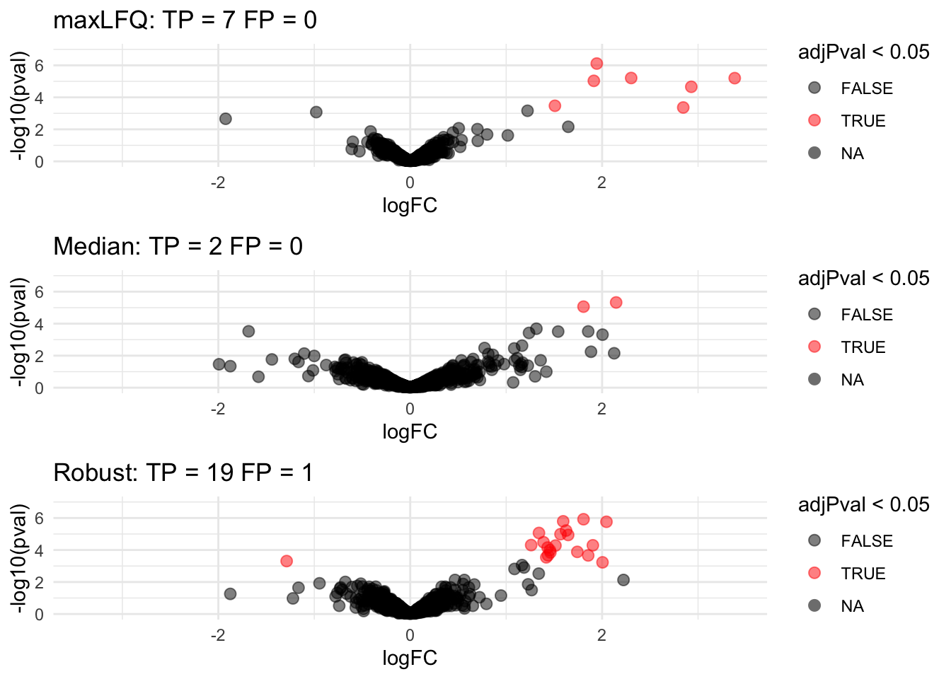

• Robust summarization: highest power and still good FDR control: \(FDP = \frac{1}{20} = 0.05\).

compBoxPlot

## Warning: Removed 1079 rows containing non-finite values (stat_boxplot).

• Median: biased logFC estimates for spike-in proteins
• maxLFQ: more variable logFC estiamtes for spike-in proteins

2.6.2 Median summarization

We first evaluate median summarization for protein P01031ups|CO5_HUMAN_UPS.

Click to see code to make plot

dataHlp <- pe[["peptideNorm"]][
    rowData(pe[["peptideNorm"]])$Proteins == prot,
    colData(pe)$lab=="lab3"] %>% assay 

sumMedian <- data.frame(
  intensity= dataHlp
    %>% colMedians(na.rm=TRUE)
  ,
  condition= colnames(dataHlp) %>% substr(12,12) %>% as.factor )

sumMedianPlot <- sumPlot + 
  geom_hline(
    data = sumMedian,
    mapping = aes(yintercept=intensity,color=condition)) + 
  ggtitle("Median summarization")

sumMedianPlot

## Warning: Removed 1 rows containing missing values (geom_hline).

• The sample medians are not a good estimate for the protein expression value.
• Indeed, they do not account for differences in peptide effects
• Peptides that ionize poorly are also picked up in samples with high spike-in concencentration and not in samples with low spike-in concentration
• This introduces a bias.

2.6.3 Mean summarization

\[ y_{ip} = \beta_i^\text{sample} + \epsilon_{ip} \]

Click to see code to make plot

sumMeanMod <- lm(intensity ~ -1 + sample,data)

sumMean <- data.frame(
  intensity=sumMeanMod$coef[grep("sample",names(sumMeanMod$coef))],
  condition= names(sumMeanMod$coef)[grep("sample",names(sumMeanMod$coef))] %>% substr(18,18) %>% as.factor )



sumMeanPlot <- sumPlot + geom_hline(
    data = sumMean,
    mapping = aes(yintercept=intensity,color=condition)) +
    ggtitle("Mean summarization")

grid.arrange(sumMedianPlot, sumMeanPlot, ncol=2)

## Warning: Removed 1 rows containing missing values (geom_hline).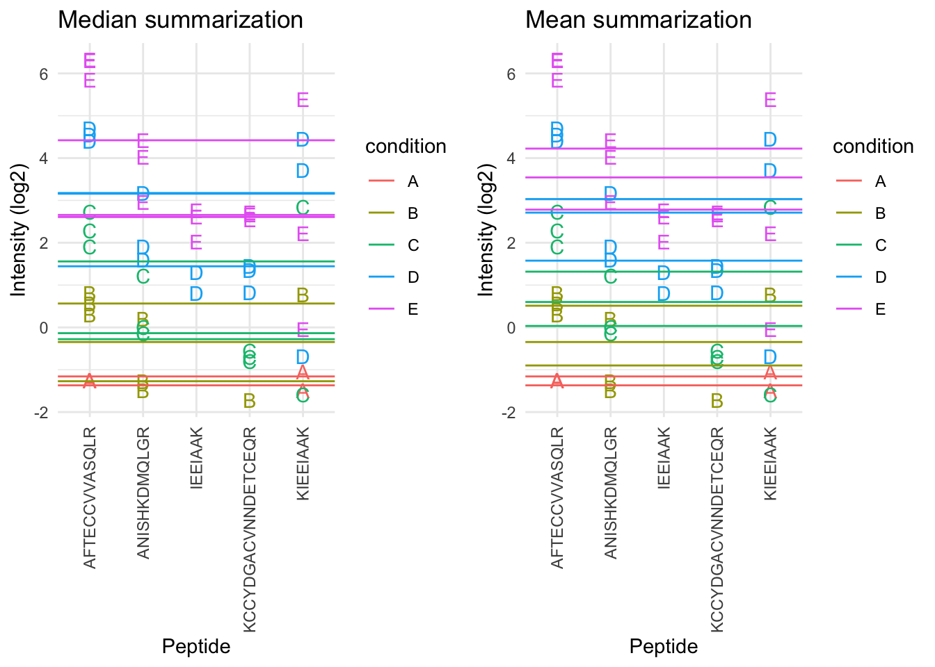

2.6.4 Model based summarization

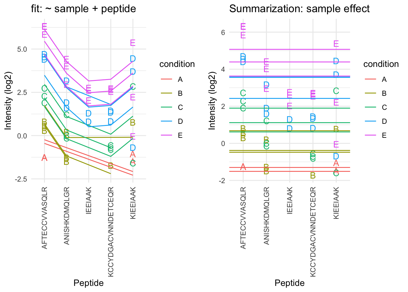
We can use a linear peptide-level model to estimate the protein expression value while correcting for the peptide effect, i.e. 

\[ y_{ip} = \beta_i^\text{sample}+\beta^{peptide}_{p} + \epsilon_{ip} \]

Click to see code to make plot

sumMeanPepMod <- lm(intensity ~ -1 + sample + peptide,data)

sumMeanPep <- data.frame(
  intensity=sumMeanPepMod$coef[grep("sample",names(sumMeanPepMod$coef))] + mean(data$intensity) - mean(sumMeanPepMod$coef[grep("sample",names(sumMeanPepMod$coef))]),
  condition= names(sumMeanPepMod$coef)[grep("sample",names(sumMeanPepMod$coef))] %>% substr(18,18) %>% as.factor )


fitLmPlot <-  sumPlot + geom_line(
    data = data %>% mutate(fit=sumMeanPepMod$fitted.values),
    mapping = aes(x=peptide, y=fit,color=condition, group=sample)) +
    ggtitle("fit: ~ sample + peptide")
sumLmPlot <- sumPlot + geom_hline(
    data = sumMeanPep,
    mapping = aes(yintercept=intensity,color=condition)) +
    ggtitle("Summarization: sample effect")

grid.arrange(sumMedianPlot, sumMeanPlot, sumLmPlot, nrow=1)

## Warning: Removed 1 rows containing missing values (geom_hline).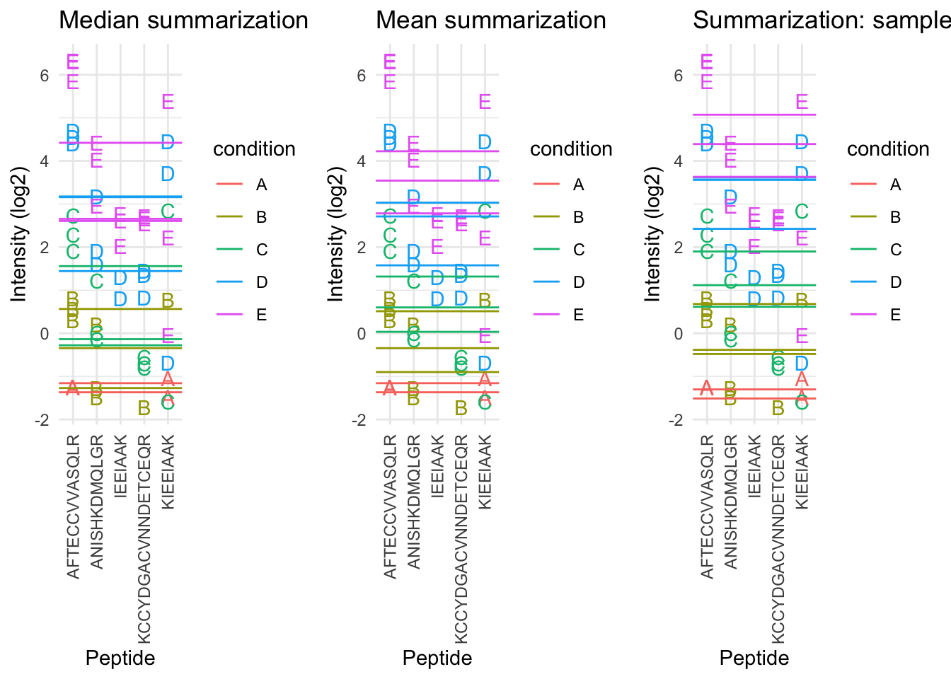

• By correcting for the peptide species the protein expression values are much better separated an better reflect differences in abundance induced by the spike-in condition.

• Indeed, it shows that median and mean summarization that do not account for the peptide effect indeed overestimate the protein expression value in the small spike-in conditions and underestimate that in the large spike-in conditions.

• Still there seem to be some issues with samples that for which the expression values are not well separated according to the spike-in condition.

A residual analysis clearly indicates potential issues:

Click to see code to make plot

resPlot <- data %>% 
  mutate(res=sumMeanPepMod$residuals) %>%
  ggplot(aes(x = peptide, y = res, color = condition, label = condition), show.legend = FALSE) +
  geom_point(shape=21) +
  theme_minimal() +
  theme(axis.text.x = element_text(angle = 90, vjust = 0.5, hjust = 1)) +
  xlab("Peptide") + 
  ylab("residual") +
  ggtitle("residuals: ~ sample + peptide")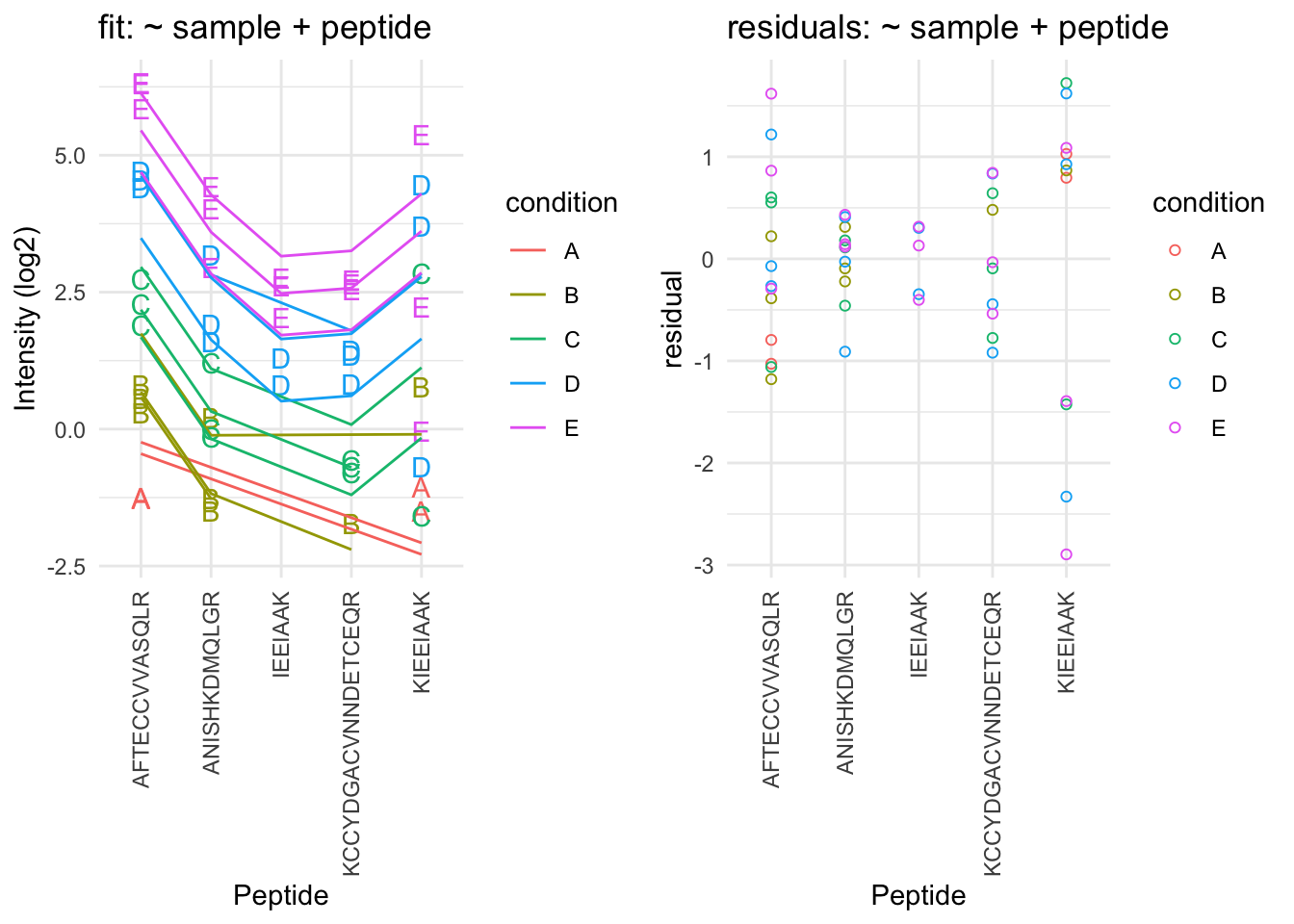

grid.arrange(fitLmPlot, resPlot, nrow = 1)

grid.arrange(fitLmPlot, sumLmPlot, nrow = 1)

• The residual plot shows some large outliers for peptide KIEEIAAK.
• Indeed, in the original plot the intensities for this peptide do not seem to line up very well with the concentration.
• This induces a bias in the summarization for some of the samples (e.g. for D and E)

2.6.5 Robust summarization using a peptide-level linear model

\[ y_{ip} = \beta_i^\text{sample}+\beta^{peptide}_{p} + \epsilon_{ip} \]

• Ordinary least squares: estimate \(\beta\) that minimizes \[ \text{OLS}: \sum\limits_{i,p} \epsilon_{ip}^2 = \sum\limits_{i,p}(y_{ip}-\beta_i^\text{sample}-\beta_p^\text{peptide})^2 \]

We replace OLS by M-estimation with loss function \[ \sum\limits_{i,p} w_{ip}\epsilon_{ip}^2 = \sum\limits_{i,p}w_{ip}(y_{ip}-\beta_i^\text{sample}-\beta_p^\text{peptide})^2 \]

• Iteratively fit model with observation weights \(w_{ip}\) until convergence
• The weights are calculated based on standardized residuals

Click to see code to make plot

sumMeanPepRobMod <- MASS::rlm(intensity ~ -1 + sample + peptide,data)
resRobPlot <- data %>%
  mutate(res = sumMeanPepRobMod$residuals,
         w = sumMeanPepRobMod$w) %>%
  ggplot(aes(x = peptide, y = res, color = condition, label = condition,size=w), show.legend = FALSE) +
  geom_point(shape=21,size=.2) +
  geom_point(shape=21) +
  theme_minimal() +
  theme(axis.text.x = element_text(angle = 90, vjust = 0.5, hjust = 1)) +
  xlab("Peptide") + 
  ylab("residual") + 
  ylim(c(-1,1)*max(abs(sumMeanPepRobMod$residuals)))
weightPlot <- qplot(
  seq(-5,5,.01), 
  MASS::psi.huber(seq(-5,5,.01)),
  geom="path") +
  xlab("standardized residual") +
  ylab("weight")

grid.arrange(weightPlot,resRobPlot,nrow=1)

• We clearly see that the weights in the M-estimation procedure will down-weight errors associated with outliers for peptide KIEEIAAK.

Click to see code to make plot

sumMeanPepRob <- data.frame(
  intensity=sumMeanPepRobMod$coef[grep("sample",names(sumMeanPepRobMod$coef))] + mean(data$intensity) - mean(sumMeanPepRobMod$coef[grep("sample",names(sumMeanPepRobMod$coef))]),
  condition= names(sumMeanPepRobMod$coef)[grep("sample",names(sumMeanPepRobMod$coef))] %>% substr(18,18) %>% as.factor )

sumRlmPlot <- sumPlot + geom_hline(
    data=sumMeanPepRob,
    mapping=aes(yintercept=intensity,color=condition)) + 
    ggtitle("Robust")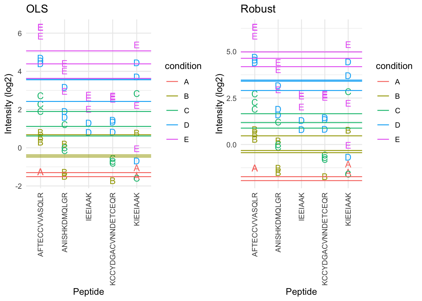

 grid.arrange(sumLmPlot + ggtitle("OLS"), sumRlmPlot, nrow = 1)

• Robust regresion results in a better separation between the protein expression values for the different samples according to their spike-in concentration.

2.6.6 Comparison summarization methods

• maxLFQ

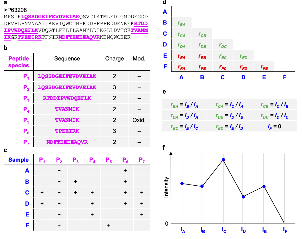
• MS-stats also uses a robust peptide level model to perform the summarization, however, they typically first impute missing values

• Proteus high-flyer method: mean of three peptides with highest intensity

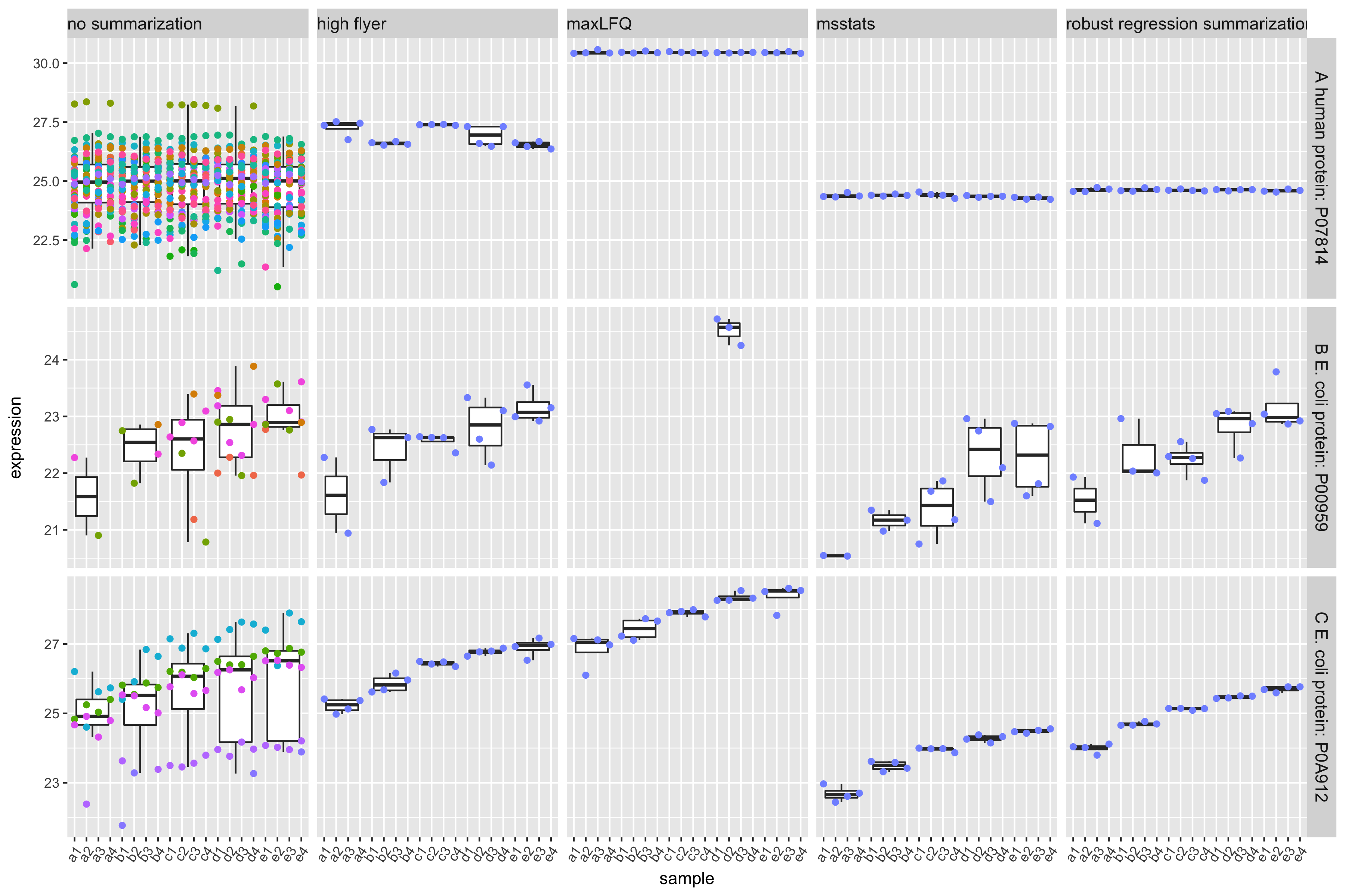
• (Sticker et al. 2020)
• doi: https://doi.org/10.1074/mcp.RA119.001624
  
• pdf

References

Sticker, A., L. Goeminne, L. Martens, and L. Clement. 2020. “Robust Summarization and Inference in Proteome-wide Label-free Quantification.” Mol Cell Proteomics 19 (7): 1209–19.