Introduction to TargetDecoy

library(TargetDecoy)
library(ggplot2)

Basics

Installing `TargetDecoy`

TargetDecoy is an R package available via the Bioconductor repository for packages. R can be installed on any operating system from CRAN after which you can install TargetDecoy by using the following commands in your R session:

if (!requireNamespace("BiocManager", quietly = TRUE)) {
      install.packages("BiocManager")
  }

BiocManager::install("TargetDecoy")

## Check that you have a valid Bioconductor installation
BiocManager::valid()

The latest development version of TargetDecoy can be installed from GitHub by running the following in an R session:

BiocManager::install("statOmics/TargetDecoy")

Citing `TargetDecoy`

We hope that TargetDecoy will be useful for your research. Please use the following information to cite the package and the overall approach. Thank you!

## Citation info
citation("TargetDecoy")
#> 
#> To cite package 'TargetDecoy' in publications use:
#> 
#>   Debrie E, Clement L, Malfait M (2022). _TargetDecoy: Diagnostic Plots
#>   to Evaluate the Target Decoy Approach_.
#>   https://www.bioconductor.org/packages/TargetDecoy,
#>   https://statomics.github.io/TargetDecoy/,
#>   https://github.com/statOmics/TargetDecoy/.
#> 
#> A BibTeX entry for LaTeX users is
#> 
#>   @Manual{,
#>     title = {TargetDecoy: Diagnostic Plots to Evaluate the Target Decoy Approach},
#>     author = {Elke Debrie and Lieven Clement and Milan Malfait},
#>     year = {2022},
#>     note = {https://www.bioconductor.org/packages/TargetDecoy,
#> https://statomics.github.io/TargetDecoy/,
#> https://github.com/statOmics/TargetDecoy/},
#>   }

Introduction

A first step in the data analysis of Mass Spectrometry (MS) based proteomics data is to identify peptides and proteins. For this, a huge number of experimental mass spectra typically have to be assigned to theoretical peptides derived from a sequence database. This task is carried out by specialised algorithms called search engines, which compare each of the observed spectra to theoretical spectra derived from relevant candidate peptides obtained from a sequence data base and calculate a score for each comparison. The observed spectrum is then assigned to the theoretical peptide with the best score, which is also referred to as a peptide-to-spectrum match (PSM). It is of course crucial for the downstream analysis to evaluate the overall reliability of these matches. Therefore False Discovery Rate (FDR) control is used to return a sufficiently reliable list of PSMs. The FDR calculation, however, requires a good characterisation of the score distribution of PSMs that are matched to an incorrect peptide (bad target hits). In proteomics, the target decoy approach (TDA) is typically used for this purpose. The TDA method matches the observed spectra to a database of real (target) and nonsense (decoy) peptides, with the latter typically generated by reversing protein sequences in the target database. Hence, all PSMs that match to a decoy peptide are known to be bad hits and the distribution of their scores is used to estimate the distribution of the bad scoring target PSMs. A crucial assumption of the TDA is that decoy PSM hits have similar properties as bad target hits so that decoy PSM scores are a good simulation of target PSM scores. Users, however, typically do not evaluate these assumptions. To this end we developed TargetDecoy to generate diagnostic plots to evaluate the quality of the target decoy method, thus allowing users to assess whether the key assumptions underlying the method are met.

Concepts

Basic Statistical Concepts

We first introduce some notation. With \(x\) we denote the PSM and without loss of generality we assume that larger score values indicate a better match to the theoretical spectrum. The scores will follow a mixture distribution:

\[f(x) = \pi_0f_0(x)+(1-\pi_0)f_1(x),\]

with \(f(x)\) the target PSM score distribution, \(f_0(x)\) the mixture component corresponding to incorrect PSMs, \(f_1(x)\) the mixture component corresponding to the correct PSMs and \(\pi_0\) the fraction of incorrect PSMs. Based on the mixture distribution we can calculate the posterior probability that a PSM with score \(x\) is a bad match:

\[ P[\text{Bad hit} \mid \text{score }x]=\frac{\pi_0 f_0 (x)}{f(x)}, \]

which is also referred to as the posterior error probability (PEP) in mass spectrometry based proteomics. With the mixture model, we can also calculate the posterior probability that a random PSM in the set of all PSMs with scores above a score threshold t is a bad hit:

\[ P[\text{Bad hit} \mid \text{score }x>t]=\pi_0 \frac{\int\limits_{x=t}^{+\infty} f_0(x)dx}{\int\limits_{x=t}^{+\infty} f(x)dx}, \]

with \(\int\limits_{x=t}^{+\infty} f_0(x) dx\) the probability to observe a bad PSM hit above the threshold and, \(\int\limits_{x=t}^{+\infty} f(x) dx\) the probability to observe a target PSM hit above the threshold. The probability \(P[\text{Bad hit} \mid \text{score }x>t]\) is also referred to as the False Discovery Rate for peptide identification (FDR) of the set of PSMs with scores above the threshold \(t\). Hence, the FDR has the interpretation of the expected fraction of bad hits in the set of all target hits that are returned in the final PSM list, so bad PSM hits with scores above the threshold.

In order to estimate the FDR, we thus have to estimate the distribution of the bad hits and of the targets. In proteomics this is typically done by the use of the Target Decoy Approach (TDA).

Target Decoy Approach

A competitive target decoy search involves performing a search on a concatenated target and decoy database (as, for example, obtained from a reversed target database). Typically, one will ensure that there are as many targets as there are decoys. If the decoy hits are a good simulation of the bad target hits, it is equally likely that a bad hit will go to the targets as as it is to go to the decoys. With a competitive target decoy approach, it is therefore assumed that a bad hit matches a bad target equally likely as a decoy.

The distribution of bad target hits (\(f_0(t)\)) and the marginal distribution of all target hits (\(f(t)\)) is empirically estimated using the decoy scores and all target scores respectively. With the TDA, the FDR of the set of returned PSMs with scores above a threshold t, is estimated by dividing the number of decoy hits with a score above t by the number of target PSMs with a score above t.

\[ \widehat{\text{FDR}}(t) = \frac{\#\widehat{\text{ bad hits}} \mid x>t}{\#\text{ targets} \mid x>t} \stackrel{(*)}{=} \frac{\#\text{ decoys} \mid x>t}{\#\text{ targets} \mid x>t} \\ (*) \text{ Assumption TDA}: \text{bad targets} \stackrel{d}{=} \text{decoys} \]

This can be rewritten as:

\[\widehat{\text{FDR}}(t)=\frac{\#decoys}{\#targets} \cdot \frac{\frac{\# decoys \mid x>t}{\#decoys}}{\frac{\#targets \mid x>t}{\#targets}}\]

\[\widehat{\text{FDR}}(t) = {\widehat{\pi}}_0 \frac{\widehat{\int\limits_t^{+\infty} f_0(x) dx}}{\widehat{\int\limits_t^{+\infty} f(x)dx}}\]

Hence, the proportion of bad hits \(\pi_0\) is estimated as the number of decoys divided by the number of targets, since the competitive TDA assumes that it is equally likely that a bad hit matches to a bad target hit or to a decoy. The probability on a (bad) target PSM hit above the threshold is estimated based on the empirical cumulative distribution in the sample, i.e. as the fraction of targets (decoys) that are above the threshold. Hence, a second assumption is that the decoy scores provide a good simulation of the bad target scores.

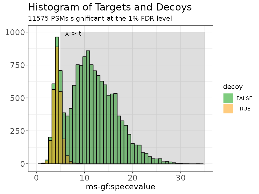
Illustration of the target and decoy distributions. The green bars are the histogram of the target PSM scores. The orange bars are the histogram of the decoy PSM scores. We see that the decoy PSMs match well with the incorrect target hits that are more likely to occur at low scores.

In summary, two assumptions have to be checked:

Assumption 1: The decoy PSM hits are a good simulation of the bad target hits and the distributions are equal.
Assumption 2: When the library size of targets and decoys is the same, it is equally likely that a bad hit matches to a target sequence or to a decoy sequence.

When these two assumptions are met we can replace the number of bad hits by the number of decoys.

These assumptions can be checked using a histogram and a PP-plot.

Diagnostic plots

Histogram

In the histogram the shape of the score distribution of the decoys (shown in blue in the figure below) should be equal to that of bad target hits (first mode in the target distribution indicated in red). Note that the height of the decoys can be slightly lower than the first mode in the target distribution because some good target hits also have a low score (e.g., because of poor quality observed spectra).

data("ModSwiss")
evalTargetDecoysHist(ModSwiss,
    decoy = "isdecoy", score = "ms-gf:specevalue",
    log10 = TRUE, nBins = 50
)

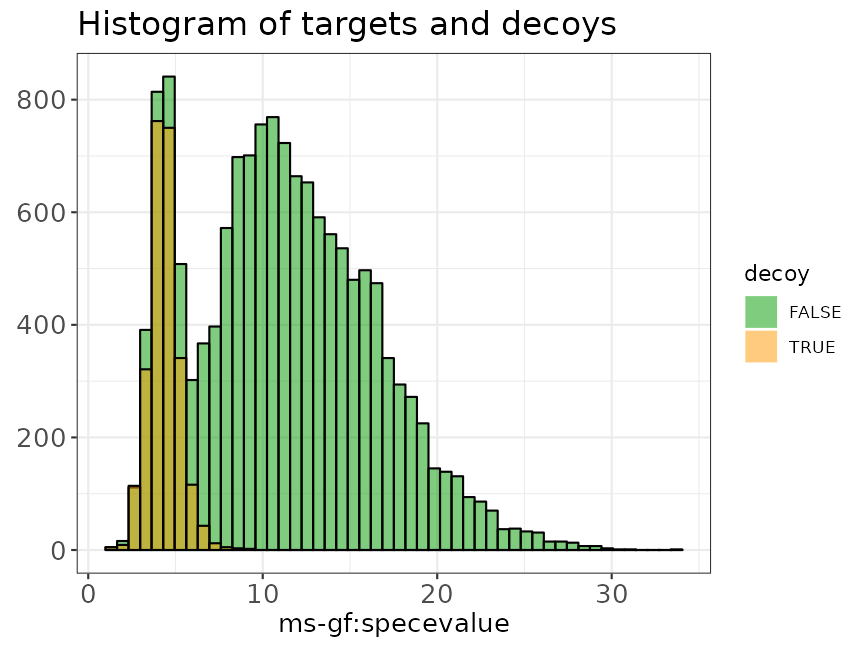
Histogram of the scores of targets and decoys.

PPplot

The figure below shows an example of a PP plot, the main diagnostic plot to evaluate the quality of the decoys.

evalTargetDecoysPPPlot(ModSwiss,
    decoy = "isdecoy", score = "ms-gf:specevalue",
    log10 = TRUE
)

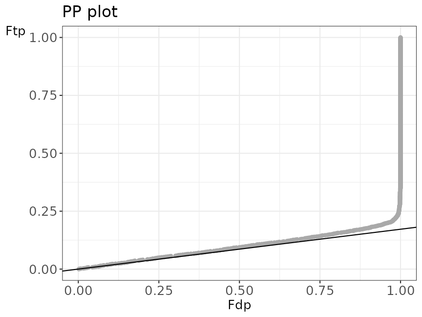
PP plot

Deviations from the assumptions of TDA can be best evaluated in the PP-plot. The PP-plot displays the empirical cumulative distribution (ECDF) from the target distribution in function of that of the decoy distribution. PP-plots have the property that they show a straight 45 degree line through the origin if and only if both distributions are equivalent. Any deviation from this straight line indicates that the distributions differ. Note that we expect that these distributions will differ for targets and decoys. Indeed, the target distribution is stochastically larger than the decoy distribution as larger scores indicate more reliable hits and as decoys are believed to behave similarly to bad target hits. Hence, the PP-plot for targets versus decoys will always be expected to lie below the 45 degree line. When the decoys are a good simulation for the bad target hits, however, the lower values in the PP-plot should lie on a straight line through the origin with a slope determined by \(\widehat{\pi}_0\). Indeed, small target PSM scores are most likely bad hits. Hence we will include the \(\widehat{\pi}_0\)-line in our diagnostic PP plot to evaluate the quality of the decoys.

When the assumptions of the TDA approach are violated, the dots in the PP-plot at lower percentiles will deviate from the \(\widehat{\pi}_0\) line. In case the PP-plot is still a straight line at lower percentiles, then the shape of the decoy distribution is correct, but there are less (or more) decoys than expected under the concatenated TDA assumption, which could occur if the decoy database is different in size than the target database or when a bad hit is less likely to match to a decoy than to a bad target hit. This would also be visible in the histograms: the decoy histogram would be considerably lower (higher) than the first mode of the target distribution. When the PP-plot at lower percentiles deviates from a straight line, the distribution of decoys and the bad target PSMs is not equivalent, indicating that the decoys are not a good simulation of bad target hits. Either type of deviation should be of concern as each indicates that the FDR returned by the conventional concatenated TDA is incorrect.

Supported data formats

TargetDecoy currently supports objects of class mzID or mzRIdent from the mzID and mzR packages, respectively.

These datasets are typically loaded from an .mzid file as follows

filename <- system.file("extdata/55merge_omssa.mzid", package = "mzID")

## mzID
mzID_object <- mzID::mzID(filename)
#> reading 55merge_omssa.mzid... DONE!
class(mzID_object)
#> [1] "mzID"
#> attr(,"package")
#> [1] "mzID"

## mzRIdent
mzR_object <- mzR::openIDfile(filename)
class(mzR_object)
#> [1] "mzRident"
#> attr(,"package")
#> [1] "mzR"

Examples

The data

In this vignette we use data from a Pyrococcus furiosis sample run on a LTQ-Orbitrap Velos mass spectrometer. The data can be found in the PRIDE repository with identifier PXD001077. The Pyrococcus furiosis reference proteome fasta files were downloaded from UniProtKB and UniProtKB/Swiss-Prot on April 22, 2016. The Pyrococcus data was searched against all Pyrococcus proteins with multiple search engines using either the reference proteome from UniProtKB or the reference proteome from UniProtKB/Swiss-Prot.

This dataset is available in the TargetDecoy installation and can be loaded with data("ModSwiss").

Example 1: One file and one search engine

Example 1.1: MSGF+ search engine

In the next example MS-GF+ was used as the database search engine and SwissProt was used as protein sequence database. The MS-GF+ search provided an mzid file.

## Load the example SwissProt dataset
data("ModSwiss")

We use the function evalTargetDecoys(). This function creates two diagnostic plots, i.e. a histogram and a PP plot. It can be used to evaluate the quality of the target decoy approach, i.e. to check the competitive TDA assumptions.

It has the following arguments:

object: mzID object, mzR object or data.frame
decoy: Character, name of the decoy variable which consists of a boolean that indicates if the score belongs to a target or a decoy. Name of this variable in the file (typically "isdecoy" or "isDecoy").
score: Score variable contains the scores of the search engine, which have to be continuous (larger scores are assumed to be better. E-values are typically -log10(e-value) transformed.) Name of the variable depends on the search engine.
log10: Logical. Should the score be log10 transformed? Typically used when the score is an e-value. The default is TRUE.
nBins: Number of bins in the histogram. The default is 50

evalTargetDecoys() will return a figure consisting of 4 plots:

A PP plot showing the empirical cumulative distribution of the target distribution in function of that of the decoy distribution
A histogram showing the score distributions of the decoys and non-decoys
A zoomed PP plot
A zoomed histogram

evalTargetDecoys(ModSwiss,
    decoy = "isdecoy", score = "ms-gf:specevalue",
    log10 = TRUE, nBins = 50
)

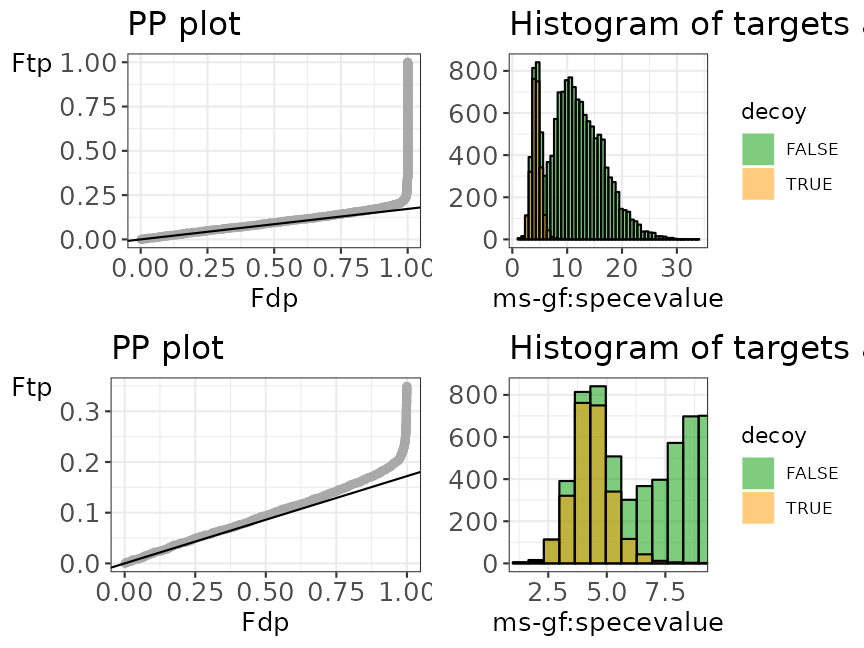
Histogram and PP plot, as well as a zoom for both plots.

The four plots can also be generated individually as follows:

msgfSwiss_ppPlot <- evalTargetDecoysPPPlot(ModSwiss,
    decoy = "isdecoy", score = "ms-gf:specevalue",
    log10 = TRUE
)
msgfSwiss_ppPlot_zoomed <- evalTargetDecoysPPPlot(ModSwiss,
    decoy = "isdecoy", score = "ms-gf:specevalue",
    log10 = TRUE, zoom = TRUE
)
msgfSwiss_hist <- evalTargetDecoysHist(ModSwiss,
    decoy = "isdecoy", score = "ms-gf:specevalue",
    log10 = TRUE, nBins = 50
)
msgfSwiss_hist_zoomed <- evalTargetDecoysHist(ModSwiss,
    decoy = "isdecoy", score = "ms-gf:specevalue",
    log10 = TRUE, nBins = 50, zoom = TRUE
)

All plots are ggplot objects, which means that one can zoom in on any part of the plot.

msgfSwiss_ppPlot +
    coord_cartesian(xlim = c(NA, 0.25), ylim = c(NA, 0.05))
#> Coordinate system already present. Adding new coordinate system, which will replace the existing one.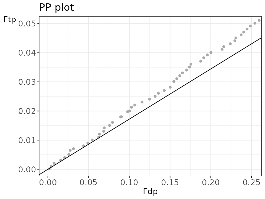

Zoom of the first part of the PP plot

Interpretation

The histogram shows that the shape of the distribution of the decoys (shown in blue) is approximately equal to that of the bad target hits (first mode in the target distribution indicated in red). The height of the decoys is slightly lower than the first mode in the target distribution, which is due to the fact that some good target hits also have a low score. This indicates that the form is good which is also confirmed in the PP-plot.

Moreover, the first part of the PP-plot is linear with a slope that is about equal to \(\hat{\pi}_0\) line. This indicates that the decoy distribution and the mixture component for incorrect PSMs of the target mixture distribution (= distribution of the bad target hits) coincide more or less. This profile in the PP-plot indicates that the set of decoys from the complete search is representative for the bad target hits. Hence, the assumptions of the concatenated TDA approach are not violated for this Pyrococcus example, assumption 2 is also fulfilled.

Overall we can conclude that in this example the assumptions for the TDA are met.

Example 1.2: X!Tandem search engine

In the next example, X!Tandem was used as the database search engine and SwissProt was used as protein sequence database. The X!Tandem search provided an mzid file.

## Load X!Tandem example data
data("ModSwissXT")

We run evalTargetDecoys() with the necessary arguments.

evalTargetDecoys(ModSwissXT,
    decoy = "isdecoy", score = "x!tandem:expect",
    log10 = TRUE, nBins = 50
)

Histogram and PP plot, each with a zoom level.

The shape of the decoy distribution seems to be fine, i.e. the first part of the PP-plot lies on a straight line. But, the histogram and the PP-plot show issues with the estimation of pi0. The total number of decoys does not seem to be a good estimate for the total number of bad target PSM hits. Indeed, it seems to be more likely that a bad match is a target than a decoy! This is due to the two pass search strategy that is performed by X!tandem. In the first phase a rapid search is performed, which does not allow for modifications nor for miss cleavages. In a second phase, a new search is conducted solely against the identified peptides in the first phase, but now by using a more complex strategy that allows for missed cleavages and post translational modifications. Performing the refined search against the smaller population of candidate peptides from the first phase greatly reduces the computational complexity, however, it comes at the cost that the TDA assumptions are violated. Indeed, in the second pass low scoring PSMs can switch to a modified PSM, which seems to be the case for many decoy hits from the first phase. Many of these switched to modified target PSMs, however, remain to have a relative low score and are likely to be bad target PSMs. The number of decoy matches is no longer representative for the number of bad target matches. This example shows that the use of a second pass strategy can be very detrimental for the FDR estimation using the TDA approach.

Example 2: One file and search performed by an engine that combines different search engines

In the following example multiple database search engines where used to process the same mzID file and both Swissprot and Uniprot were used as protein sequence database. Three search engines – MS-GF+, OMSSA and X!Tandem – and a combination of these 3 (by using PeptideShaker) were used to search against both protein sequence databases. createPPlotScores() provides the possibility to evaluate each of the sub-engines and the overall itself. Two PP plots are created to evaluate the quality of the TDA.

Provide following arguments in the function. When one are more are missing, also here a GUI pops up.

object: mzID object, mzR object or data.frame
decoy: Character, name of the decoy variable which consists of a boolean that indicates if the score belongs to a target or a decoy. Name of this variable in the file (typically "isdecoy" or "isDecoy").
scores: Character vector indicating the score variables containing the scores of the search engine. Name of the variable depends on the search engine.
log10: Vector, should the score be log10 transformed? Typically used when the score is an e-value.

We will reuse the ModSwissXT object from before.

## Run createPPlotScores with necessary arguments
## Omitting 'decoy', 'scores' or 'log10' will launch the Shiny app
createPPlotScores(ModSwissXT,
    decoy = "isdecoy",
    scores = c("omssa:evalue", "ms-gf:specevalue",
               "x!tandem:expect", "peptideshaker psm score"),
    ## We can choose to log-transform some scores but not others
    log10 = c(TRUE, TRUE, TRUE, FALSE)
)

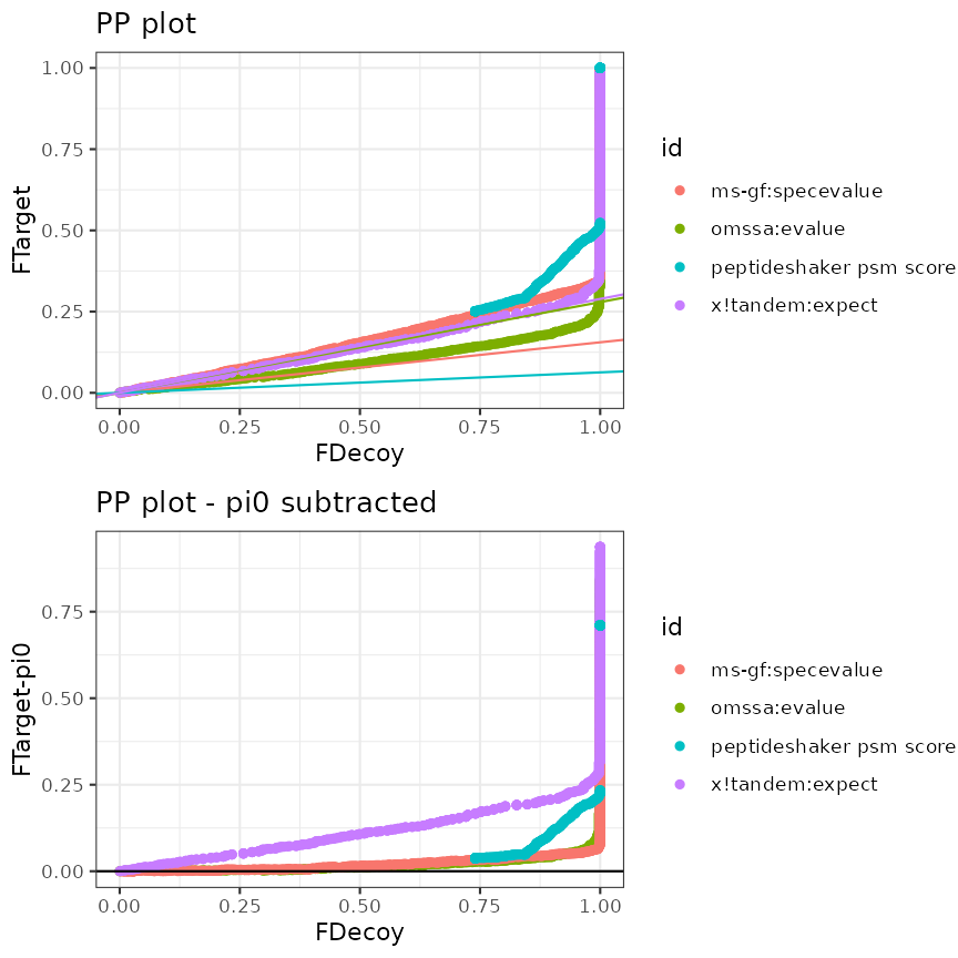
PP plot and standardized PP plot

Interpretation of the plots

For files with results for multiple search engines, a “standardized” PP-plot is also included. In this plot the estimated \(\pi_0\) is removed from the PP-plot. In the standardized PP-plot deviations in the first part have to be compared to the 0 line, which allows the user to quickly spot issues when the results of multiple search engines is visualised. The standardized plots show that the TDA assumptions hold for both MSGF+ and OMSSA. For X!tandem, however, we again see issues for the Swissprot search and these also seem to affect the combined peptide shaker search engine score that relies on all three searches.

From these plots we can deduce that combined search engines are useful. However, it is crucial to assess the TDA assumptions, otherwise the FDR control can be dramatically compromised and our tool can help data analysts to choose the engines that they include in combined search engines, carefully.

Example 3: Check the assumptions for multiple searches/runs

When you have to evaluate the quality of the TDA for different runs, it can be useful to see at a glance which runs have problems with these assumptions. The function createPPlotObjects() generated multiple files at once and two PP plots to check the necessary assumptions. A first plot with the original PP plots and pi0 lines. A second “standardized” plot where the reference \(\pi_O\) line is at 0. An overview in one figure ensures a quick evaluation of a large number of files. Based on this plot a more detailed analysis of the ‘anomalous’ runs can be done with evalTargetDecoys().

The function createPPlotObjects() has four arguments:

object_list: a list of mzID, mzR or data.frame objects.
decoy: Vector of characters, name of the decoy variable which consists of a boolean that indicates if the score belongs to a target or a decoy. Name of this variable in the file (typically "isdecoy" or "isDecoy").
score: Character vector indicating the score variables containing the scores of the search engine. Name of the variable depends on the search engine.
log10: Vector. Should the score be log10 transformed? Typically used when the score is an e-value.

Again, when all of these arguments are given correctly, the function will be executed and the desired plots will be created. However, if the user forgets to provide one of the arguments, or gives an incorrect variable that does not belong to the desired class, a shiny app is launched to select the variables for each input object given in object_list.

Provide a list with all objects

We will reuse the data sets from the previous examples and store them in a list.

Example 3.1: Two data sets with the same search engine

In this example scores come from the same search engine, MS-GF+, and thus are indicated by the same variable name "ms-gf:specevalue".

## Create list of input objects, list names will be reused in the plots
mzObjects <- list(
    ModSwiss_data = ModSwiss,
    pyroSwissprot_data = ModSwissXT
)

createPPlotObjects(
    mzObjects, decoy = "isdecoy",
    score = "ms-gf:specevalue"
)

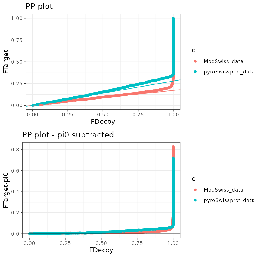
PP plot and standardized PP plot for two searches (same search engine)

Example 3.2: Two objects with different search engines

In this last example, different variable names for score are given as a vector, because two different search engines, MS-GF+ and X!tandem, were used.

## Create list of input objects, list names will be reused in the plots
mzObjects <- list(
    ModSwiss_data = ModSwiss,
    ModSwissXT_data = ModSwissXT
)

plotDiffEngine <- createPPlotObjects(mzObjects,
    decoy = "isdecoy",
    score = c("ms-gf:specevalue", "x!tandem:expect")
)
plotDiffEngine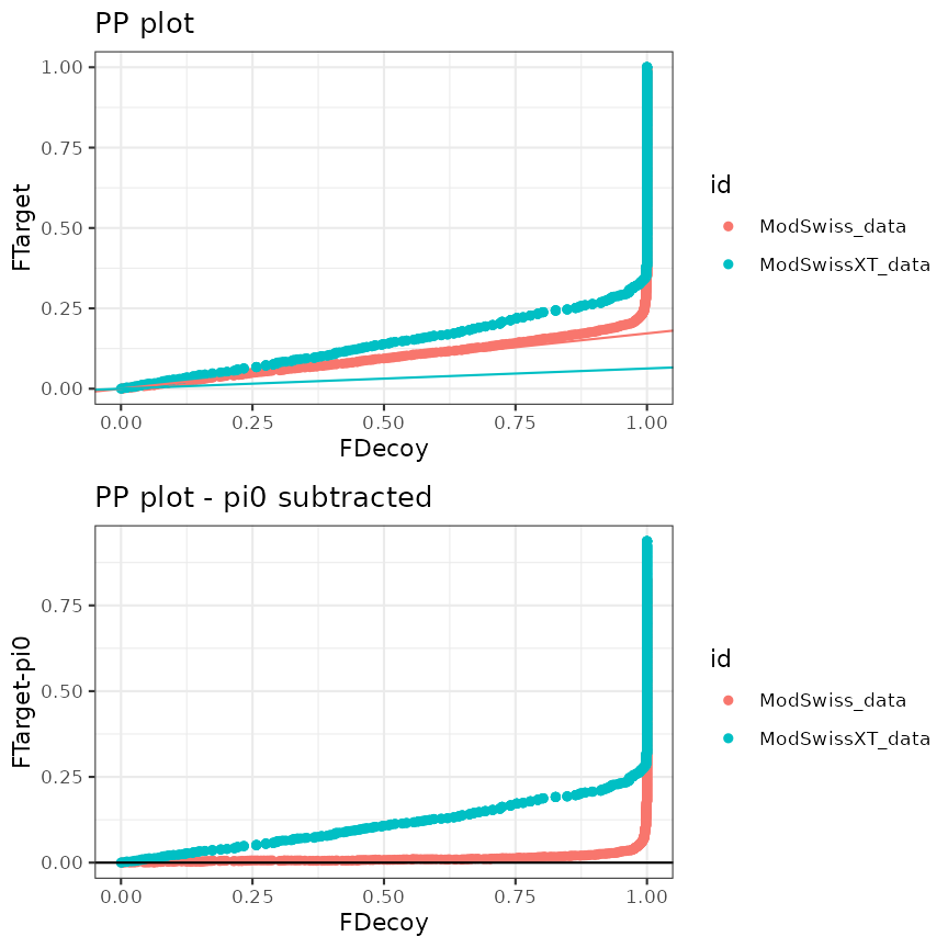

PP plot and standardized PP plot for two searches (different search engine)

Also here, it can be useful to zoom in on one specific part of the figure.

# Zoom in on the relevant or desired part of the plot
plotZoom <- plotDiffEngine +
    coord_cartesian(xlim = c(NA, 0.25), ylim = c(NA, 0.05))
#> Coordinate system already present. Adding new coordinate system, which will replace the existing one.
plotZoom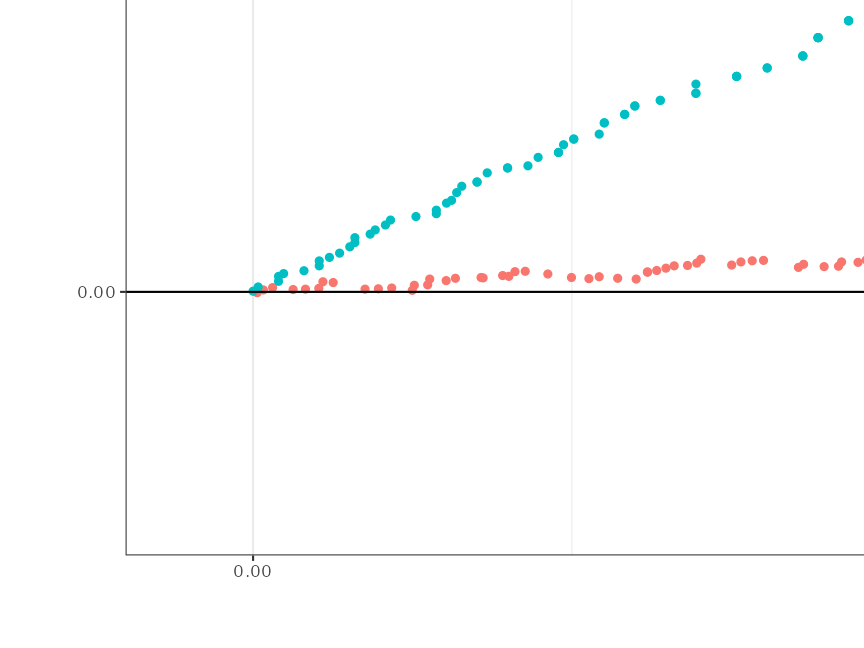

In a final step, we can investigate the anomalous plot in more detail using evalTargetDecoys().

evalTargetDecoys(mzObjects$ModSwissXT_data,
    decoy = "isdecoy", score = "x!tandem:expect",
    log10 = TRUE, nBins = 50
)

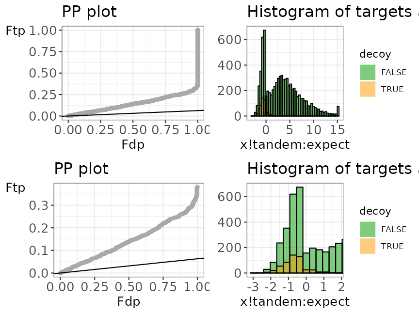
Histogram and PP plot, each with a zoom level.

Similar to example 1.2, the histogram and the PP-plot show issues with the estimation of \(\pi_0\), which is due to the second pass strategy that is performed by X!tandem.

Shiny gadget

Sometimes the variable names are not known up front. If this is the case, the ⁠evalTargetDecoys*()⁠ functions can be called with only an input object. This launches a Shiny gadget that allows selecting the variables interactively. A histogram and PP-plot of the selected variables are created on the fly for previewing, together with a snapshot of the selected data.

When working in RStudio, the gadget opens in the “Viewer” pane by default, but it can also be opened in any browser window.

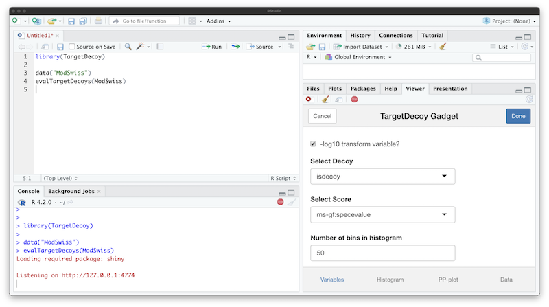
The Shiny gadget opens after calling evalTargetDecoys() with only an input object but no variables specified.

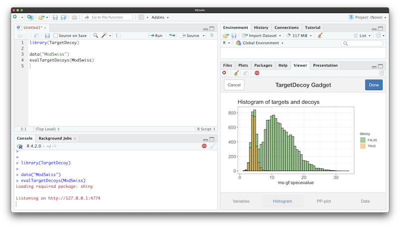
A histogram and PP-plot can be previewed in the respective tabs.

Reproducibility

R session information.

#> ─ Session info ───────────────────────────────────────────────────────────────────────────────────────────────────────
#>  setting  value
#>  version  R version 4.2.2 (2022-10-31)
#>  os       Ubuntu 20.04.5 LTS
#>  system   x86_64, linux-gnu
#>  ui       X11
#>  language en
#>  collate  C.UTF-8
#>  ctype    C.UTF-8
#>  tz       UTC
#>  date     2022-11-04
#>  pandoc   2.19.2 @ /usr/bin/ (via rmarkdown)
#> 
#> ─ Packages ───────────────────────────────────────────────────────────────────────────────────────────────────────────
#>  package      * version   date (UTC) lib source
#>  abind          1.4-5     2016-07-21 [1] RSPM
#>  backports      1.4.1     2021-12-13 [1] RSPM
#>  Biobase        2.56.0    2022-04-26 [1] Bioconductor
#>  BiocGenerics   0.42.0    2022-04-26 [1] Bioconductor
#>  BiocManager    1.30.19   2022-10-25 [1] RSPM
#>  BiocStyle    * 2.24.0    2022-04-26 [1] Bioconductor
#>  bookdown       0.29      2022-09-12 [1] RSPM
#>  broom          1.0.1     2022-08-29 [1] RSPM
#>  bslib          0.4.1     2022-11-02 [1] RSPM
#>  cachem         1.0.6     2021-08-19 [1] RSPM
#>  car            3.1-1     2022-10-19 [1] RSPM
#>  carData        3.0-5     2022-01-06 [1] RSPM
#>  cli            3.4.1     2022-09-23 [1] RSPM
#>  codetools      0.2-18    2020-11-04 [3] CRAN (R 4.2.2)
#>  colorspace     2.0-3     2022-02-21 [1] RSPM
#>  cowplot        1.1.1     2020-12-30 [1] RSPM
#>  desc           1.4.2     2022-09-08 [1] RSPM
#>  digest         0.6.30    2022-10-18 [1] RSPM
#>  doParallel     1.0.17    2022-02-07 [1] RSPM
#>  dplyr          1.0.10    2022-09-01 [1] RSPM
#>  ellipsis       0.3.2     2021-04-29 [1] RSPM
#>  evaluate       0.17      2022-10-07 [1] RSPM
#>  fansi          1.0.3     2022-03-24 [1] RSPM
#>  farver         2.1.1     2022-07-06 [1] RSPM
#>  fastmap        1.1.0     2021-01-25 [1] RSPM
#>  foreach        1.5.2     2022-02-02 [1] RSPM
#>  fs             1.5.2     2021-12-08 [1] RSPM
#>  generics       0.1.3     2022-07-05 [1] RSPM
#>  ggplot2      * 3.3.6     2022-05-03 [1] RSPM
#>  ggpubr         0.4.0     2020-06-27 [1] RSPM
#>  ggsignif       0.6.4     2022-10-13 [1] RSPM
#>  glue           1.6.2     2022-02-24 [1] RSPM
#>  gtable         0.3.1     2022-09-01 [1] RSPM
#>  highr          0.9       2021-04-16 [1] RSPM
#>  htmltools      0.5.3     2022-07-18 [1] RSPM
#>  httpuv         1.6.6     2022-09-08 [1] RSPM
#>  iterators      1.0.14    2022-02-05 [1] RSPM
#>  jquerylib      0.1.4     2021-04-26 [1] RSPM
#>  jsonlite       1.8.3     2022-10-21 [1] RSPM
#>  knitr        * 1.40      2022-08-24 [1] RSPM
#>  labeling       0.4.2     2020-10-20 [1] RSPM
#>  later          1.3.0     2021-08-18 [1] RSPM
#>  lifecycle      1.0.3     2022-10-07 [1] RSPM
#>  magrittr       2.0.3     2022-03-30 [1] RSPM
#>  memoise        2.0.1     2021-11-26 [1] RSPM
#>  mime           0.12      2021-09-28 [1] RSPM
#>  miniUI         0.1.1.1   2018-05-18 [1] RSPM
#>  munsell        0.5.0     2018-06-12 [1] RSPM
#>  mzID           1.34.0    2022-04-26 [1] Bioconductor
#>  mzR            2.30.0    2022-04-26 [1] Bioconductor
#>  ncdf4          1.19      2021-12-15 [1] RSPM
#>  pillar         1.8.1     2022-08-19 [1] RSPM
#>  pkgconfig      2.0.3     2019-09-22 [1] RSPM
#>  pkgdown        2.0.6     2022-07-16 [1] any (@2.0.6)
#>  plyr           1.8.7     2022-03-24 [1] RSPM
#>  promises       1.2.0.1   2021-02-11 [1] RSPM
#>  ProtGenerics   1.28.0    2022-04-26 [1] Bioconductor
#>  purrr          0.3.5     2022-10-06 [1] RSPM
#>  R6             2.5.1     2021-08-19 [1] RSPM
#>  ragg           1.2.4     2022-10-24 [1] RSPM
#>  Rcpp           1.0.9     2022-07-08 [1] RSPM
#>  rlang          1.0.6     2022-09-24 [1] RSPM
#>  rmarkdown      2.17      2022-10-07 [1] RSPM
#>  rprojroot      2.0.3     2022-04-02 [1] RSPM
#>  rstatix        0.7.0     2021-02-13 [1] RSPM
#>  sass           0.4.2     2022-07-16 [1] RSPM
#>  scales         1.2.1     2022-08-20 [1] RSPM
#>  sessioninfo    1.2.2     2021-12-06 [1] any (@1.2.2)
#>  shiny          1.7.3     2022-10-25 [1] RSPM
#>  stringi        1.7.8     2022-07-11 [1] RSPM
#>  stringr        1.4.1     2022-08-20 [1] RSPM
#>  systemfonts    1.0.4     2022-02-11 [1] RSPM
#>  TargetDecoy  * 1.5.0     2022-11-04 [1] local
#>  textshaping    0.3.6     2021-10-13 [1] RSPM
#>  tibble         3.1.8     2022-07-22 [1] RSPM
#>  tidyr          1.2.1     2022-09-08 [1] RSPM
#>  tidyselect     1.2.0     2022-10-10 [1] RSPM
#>  utf8           1.2.2     2021-07-24 [1] RSPM
#>  vctrs          0.5.0     2022-10-22 [1] RSPM
#>  withr          2.5.0     2022-03-03 [1] RSPM
#>  xfun           0.34      2022-10-18 [1] RSPM
#>  XML            3.99-0.12 2022-10-28 [1] RSPM
#>  xtable         1.8-4     2019-04-21 [1] RSPM
#>  yaml           2.3.6     2022-10-18 [1] RSPM
#> 
#>  [1] /home/runner/work/_temp/Library
#>  [2] /opt/R/4.2.2/lib/R/site-library
#>  [3] /opt/R/4.2.2/lib/R/library
#> 
#> ──────────────────────────────────────────────────────────────────────────────────────────────────────────────────────

Elke Debrie

Adriaan Sticker

Milan Malfait

Lieven Clement

4 November 2022

Basics

Installing `TargetDecoy`

Citing `TargetDecoy`

Introduction

Concepts

Basic Statistical Concepts

Target Decoy Approach

Diagnostic plots

Histogram

PPplot

Supported data formats

Examples

The data

Example 1: One file and one search engine

Example 1.1: MSGF+ search engine

Interpretation

Example 1.2: X!Tandem search engine

Example 2: One file and search performed by an engine that combines different search engines

Interpretation of the plots

Example 3: Check the assumptions for multiple searches/runs

Provide a list with all objects

Example 3.1: Two data sets with the same search engine

Example 3.2: Two objects with different search engines

Shiny gadget

Reproducibility

Introduction to TargetDecoy

Elke Debrie

Adriaan Sticker

Milan Malfait

Lieven Clement

4 November 2022

Basics

Installing TargetDecoy

Citing TargetDecoy

Introduction

Concepts

Basic Statistical Concepts

Target Decoy Approach

Diagnostic plots

Histogram

PPplot

Supported data formats

Examples

The data

Example 1: One file and one search engine

Example 1.1: MSGF+ search engine

Interpretation

Example 1.2: X!Tandem search engine

Example 2: One file and search performed by an engine that combines different search engines

Interpretation of the plots

Example 3: Check the assumptions for multiple searches/runs

Provide a list with all objects

Example 3.1: Two data sets with the same search engine

Example 3.2: Two objects with different search engines

Shiny gadget

Reproducibility

Installing `TargetDecoy`

Citing `TargetDecoy`