Mixed Models for labelled proteomics:

This is part of the online course Statistical Genomics Analysis (SGA)

This chapter builds upon the introductory course to mixed models for proteomics data analysis. We will here cover more advanced concepts using msqrob2. To illustrate these advanced concepts, we will use the spike-in study published by Huang et al. (2020). We chose this data set because:

1. Spike-in data contain ground truth information about which proteins are differentially abundant, enabling us to show the impact of different analysis strategies.
2. It has been acquired with a TMT-labelling strategy that require a complex experimental design. This provides an excellent example to explain the different sources of variability in an MS experiment and demonstrate the flexibility of msqrob2 to model this variability.

1 Background

Labelling strategies in mass spectrometry (MS)-based proteomics enhance sample throughput by enabling the acquisition of multiple samples within a single run. The labelling strategy that allows the highest multiplexing is the tandem mass tag (TMT) labelling and will be the focus of the current tutorial.

1.1 TMT workflow

TMT-based workflow highly overlap with label-free workflows. However, TMT-based workflows have an additional sample preparation step, where the digested peptides from each sample are labelled with a TMT reagent and samples with different TMT reagents are pooled in a single TMT mixture. The signal processing is also slightly affected since the quantification no longer occurs in the MS1 space but at the MS2 level. It is important to understand that TMT reagent are isobaric, meaning that the same peptide with different TMT labels will have the same mass for the intact ion, as recorded during MS1. However, the TMT fragments that are released upon fragmentation during MS2, also called TMT reporter ions, have label-specific masses. The TMT fragments have an expected mass and are distributed in a low-mass range of the MS2 space. The intensity of each TMT fragment is directly proportional to the peptide quantity in the original sample before pooling. The TMT fragment intensities measured during MS2 are used as quantitative data. The higher mass range contains the peptide fragments that compose the peptide fingerprint, similarly to LFQ. This data range is therefore used for peptide identification. Interestingly, the peptide fingerprint originates from the same peptide across multiple samples. This leads to a signal boost for low abundant peptides and hence should improve data sensitivity and consistency.

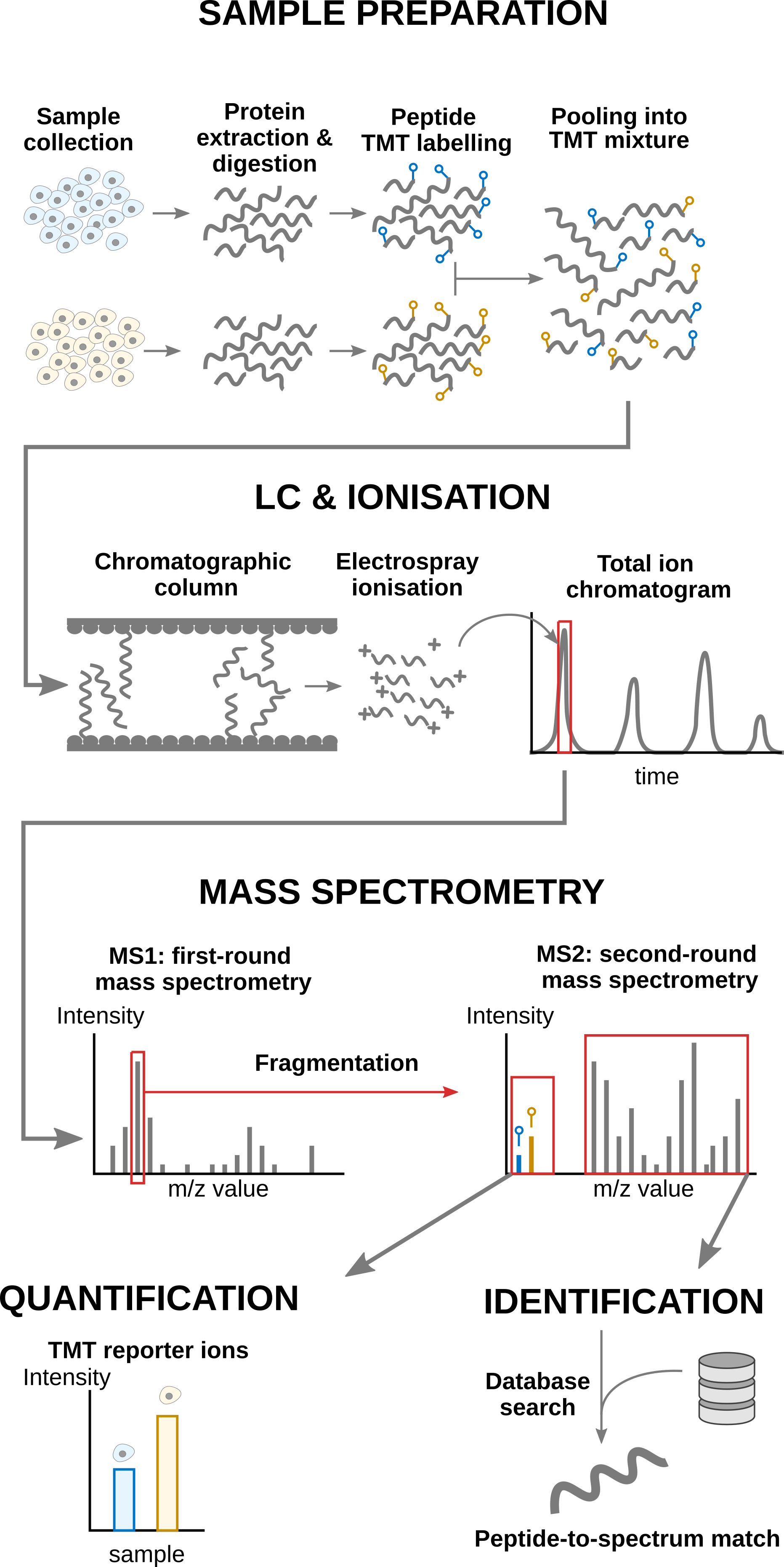
Overview of an TMT-based proteomics workflow.

1.2 Challenges

The analysis of TMT-based proteomics data shares the same challenges as the data analysis challenges for LFQ:

• MS-based proteomics doesn’t measure proteins directly, but their constituting peptide ions. The protein-level information needs to be reconstructed from the ion data. In this tutorial, we will start from the peptide data, which has been constructed from the ion data by MaxQuant.
• All peptides cannot be ionised with the same efficiency. Poor ionisation will lead to reduced signal as less ions will hit the detector, hence leading to a huge variability in intensity among different peptide species, even when they originate from the same protein.
• The identification step is not trivial and prone to errors. PSM misidentification leads to the assignment of a quantitative values from another peptide with likely another ionisation efficiency and relative abundance. Hence this misassigned value will become an outlier.
• Moreover, the ion selection for MS2 depends on its intensity (recall that only the top most intense ion peaks are send for MS2). Therefore, the chance to measure and, subsequently, identify a peptide will depend on its abundance. Non identified peptides will lead to data missingness, which is related to the underlying quantification value. This phenomenon is known as missingness not at random. Next to that, many reasons can lead to ions not being selected or identified irrespective of their quantification value leading to missingness that is not related to its quantitative value. This is referred to as missingness completely at random. The missingness issue is not negligible: only 41% of all proteins are quantified across all samples, and the number drops to 6.6% when considering peptides.
• The identification issues lead to unbalanced peptide missingness across samples, and the patterns of missing values are potentially different for every peptide, highlighting the need for an automatised solution that is robust against missing values.
• Technical variations during the experiment can lead to systematic fluctuations across samples. The most obvious reason is when different sample amounts are injected into the instruments, due to small pipetting inconsistencies for instance. However, these differences lead to unwanted variation that should be discarded when answering biological questions.
• TMT workflows impose an additional challenge. Contemporary experiments often involve increasingly complex designs, where the number of samples exceeds the capacity of a single TMT mixture, resulting in a complex correlation structure that must be addressed for accurate statistical inference. We will describe in the modelling section the different sources of variation.

1.3 Experimental context

The data set used in this chapter is a spike-in experiment (PXD0015258) published by Huang et al. (2020). It consists of controlled mixtures with known ground truth. UPS1 peptides at concentrations of 500, 333, 250, and 62.5 fmol were spiked into 50 g of SILAC HeLa peptides, each in duplicate. These concentrations form a dilution series of 1, 0.667, 0.5, and 0.125 relative to the highest UPS1 peptide amount (500 fmol). A reference sample was created by combining the diluted UPS1 peptide samples with 50g of SILAC HeLa peptides. All dilutions and the reference sample were prepared in duplicate, resulting in a total of ten samples. These samples were then treated with TMT10-plex reagents and combined before LC-MS/MS analysis. This protocol was repeated five times, each with three technical replicates, totaling 15 MS runs.

We will start from the PSM data generated by Skyline and infer protein-level differences between samples. To achieve this goal, we will apply an msqrob2TMT workflow, a data processing and modelling workflow dedicated to the analysis of TMT-based proteomics datasets. We will demonstrate how the workflow can highlight the spiked-in proteins. Before delving into the analysis, let us prepare our computational environment.

2 Load packages

We load the msqrob2 package, along with additional packages for data manipulation and visualisation.

library("msqrob2")
library("dplyr")
library("ggplot2")
library("patchwork")

We also configure the parallelisation framework.

library("BiocParallel")
register(SerialParam())

3 Data

The data have been deposited by the authors in the MSV000084264 MASSiVE repository, but we will retrieve the time stamped data from our Zenodo repository. We need 2 files: the Skyline identification and quantification table generated by the authors and the sample annotation files.

To facilitate management of the files, we download the required files using the BiocFileCache package. The chunk below will take some time to complete the first time you run it as it needs to download the (large) file locally, but will fetch the local copy the following times.

library("BiocFileCache")
bfc <- BiocFileCache()
psmFile <- bfcrpath(bfc, "https://zenodo.org/records/14767905/files/spikein1_psms.txt?download=1")
annotFile <- bfcrpath(bfc, "https://zenodo.org/records/14767905/files/spikein1_annotations.csv?download=1")

Now the files are downloaded, we can load the two tables.

3.1 PSM table

An MS experiment generates spectra. Each MS2 spectra are used to infer the peptide identity thanks to a search engine. When an observed spectrum is matched to a theoretical peptide spectrum, we have a peptide-to-spectrum match (PSM). The identification software compiles all the PSMs inside a table. Hence, the PSM data is the lowest possible level to perform data modelling.

Each row in the PSM data table contains information for one PSM (the table below shows the first 6 rows). The columns contains various information about the PSM, such as the peptide sequence and charge, the quantified value, the inferred protein group, the measured and predicted retention time and precursor mass, the score of the match, … In the case of TMT data, the quantification values are provides in multiple columns (start with "Abundance."), one for each TMT label. Regardless of TMT or LFQ experiments, the PSM table stacks the quantitative values from samples in different runs below each other.

psms <- read.delim(psmFile)
qcols <- grep("Abundance", colnames(psms), value = TRUE)

Checked	Confidence	Identifying.Node	PSM.Ambiguity	Annotated.Sequence	Modifications	Marked.as	X..Protein.Groups	X..Proteins	Master.Protein.Accessions	Master.Protein.Descriptions	Protein.Accessions	Protein.Descriptions	X..Missed.Cleavages	Charge	DeltaScore	DeltaCn	Rank	Search.Engine.Rank	m.z..Da.	MH…Da.	Theo..MH…Da.	DeltaM..ppm.	Deltam.z..Da.	Activation.Type	MS.Order	Isolation.Interference….	Average.Reporter.S.N	Ion.Inject.Time..ms.	RT..min.	First.Scan	Spectrum.File	File.ID	Abundance..126	Abundance..127N	Abundance..127C	Abundance..128N	Abundance..128C	Abundance..129N	Abundance..129C	Abundance..130N	Abundance..130C	Abundance..131	Quan.Info	Ions.Score	Identity.Strict	Identity.Relaxed	Expectation.Value	Percolator.q.Value	Percolator.PEP
False	High	Mascot (O4)	Unambiguous	[K].gFQQILAGEYDHLPEQAFYMVGPIEEAVAk.[A]	N-Term(TMT6plex); K30(TMT6plex)		1	1	P06576	ATP synthase subunit beta, mitochondrial OS=Homo sapiens GN=ATP5B PE=1 SV=3	P06576	ATP synthase subunit beta, mitochondrial OS=Homo sapiens GN=ATP5B PE=1 SV=3	0	3	1.0000	0	1	1	1270.3249	3808.960	3808.966	-1.51	-0.00192	CID	MS2	47.955590	8.7	50.000	212.2487	112815	161117_SILAC_HeLa_UPS1_TMT10_Mixture1_03.raw	F1	2548.326	3231.929	2760.839	4111.639	3127.254	1874.163	2831.423	2298.401	3798.876	3739.067	NA	90	28	21	0.0000000	0	0.0000140
False	High	Mascot (K2)	Unambiguous	[R].qYPWGVAEVENGEHcDFTILr.[N]	N-Term(TMT6plex); C15(Carbamidomethyl); R21(Label:13C(6)15N(4))		1	1	Q16181	Septin-7 OS=Homo sapiens GN=SEPT7 PE=1 SV=2	Q16181	Septin-7 OS=Homo sapiens GN=SEPT7 PE=1 SV=2	0	3	1.0000	0	1	1	920.4493	2759.333	2759.332	0.31	0.00028	CID	MS2	9.377507	8.1	3.242	164.7507	87392	161117_SILAC_HeLa_UPS1_TMT10_Mixture3_03.raw	F5	22861.765	25817.946	23349.498	29449.609	25995.929	22955.769	30578.971	30660.488	38728.853	25047.280	NA	76	24	17	0.0000001	0	0.0000003
False	High	Mascot (K2)	Unambiguous	[R].dkPSVEPVEEYDYEDLk.[E]	N-Term(TMT6plex); K2(Label); K17(Label)		1	1	Q9Y450	HBS1-like protein OS=Homo sapiens GN=HBS1L PE=1 SV=1	Q9Y450	HBS1-like protein OS=Homo sapiens GN=HBS1L PE=1 SV=1	1	3	0.9730	0	1	1	920.1605	2758.467	2758.461	2.08	0.00192	CID	MS2	38.317050	17.8	13.596	143.4534	74786	161117_SILAC_HeLa_UPS1_TMT10_Mixture3_03.raw	F5	25504.083	27740.450	25144.974	25754.579	29923.176	34097.637	31650.255	27632.692	23886.881	35331.092	NA	74	30	23	0.0000004	0	0.0000010
False	High	Mascot (F2)	Selected	[R].hEHQVMLmr.[Q]	N-Term(TMT6plex); M8(Oxidation); R9(Label:13C(6)15N(4))		1	1	Q15233	Non-POU domain-containing octamer-binding protein OS=Homo sapiens GN=NONO PE=1 SV=4	Q15233	Non-POU domain-containing octamer-binding protein OS=Homo sapiens GN=NONO PE=1 SV=4	0	4	0.5250	0	1	1	359.6898	1435.737	1435.738	-0.04	-0.00002	CID	MS2	21.390040	36.5	50.000	21.6426	6458	161117_SILAC_HeLa_UPS1_TMT10_Mixture4_02.raw	F10	13493.228	14674.490	11187.900	12831.495	13839.426	12441.353	13450.885	14777.844	13039.995	12057.121	NA	40	25	18	0.0003351	0	0.0001175
False	High	Mascot (K2)	Unambiguous	[R].dNLTLWTADNAGEEGGEAPQEPQS.[-]	N-Term(TMT6plex)		1	1	P31947	14-3-3 protein sigma OS=Homo sapiens GN=SFN PE=1 SV=1	P31947	14-3-3 protein sigma OS=Homo sapiens GN=SFN PE=1 SV=1	0	3	1.0000	0	1	1	920.0943	2758.268	2758.264	1.53	0.00141	CID	MS2	0.000000	16.7	6.723	174.1863	92950	161117_SILAC_HeLa_UPS1_TMT10_Mixture3_03.raw	F5	64582.786	50576.417	47126.037	56285.129	46257.310	52634.885	49716.850	60660.574	55830.488	40280.577	NA	38	21	14	0.0002153	0	0.0000138
False	High	Mascot (K2)	Unambiguous	[R].aLVAIGTHDLDTLSGPFTYTAk.[R]	N-Term(TMT6plex); K22(Label)		1	1	Q9NSD9	Phenylalanine–tRNA ligase beta subunit OS=Homo sapiens GN=FARSB PE=1 SV=3	Q9NSD9	Phenylalanine–tRNA ligase beta subunit OS=Homo sapiens GN=FARSB PE=1 SV=3	0	3	0.9783	0	1	1	919.8502	2757.536	2757.532	1.48	0.00136	CID	MS2	30.619960	26.7	8.958	176.4863	94294	161117_SILAC_HeLa_UPS1_TMT10_Mixture3_03.raw	F5	35404.709	31905.852	30993.941	36854.351	37506.001	25703.444	38626.598	35447.942	33788.409	32031.516	NA	46	29	22	0.0002060	0	0.0000720

There is a peculiarity with the dataset: the spectra have been identified with 2 nodes. In one node, the authors searched the SwissProt database for proteins with static modifications related to the metabolic labelling, in the other node they searched the Sigma_UPS protein database without these static modifications. However, some spectra were identified by both nodes leading to duplicate PSMs. We here remove these duplicated PSMs that are identification artefacts.

duplicatesQuants <- duplicated(psms[, qcols]) | duplicated(psms[, qcols], fromLast = TRUE)
psms <- psms[!duplicatesQuants, ]

We will also subset the data set to reduce computational costs. If you want to run the analysis on the full data set, you can skip this code chunk. The subsetting will keep all UPS proteins, known to be differentially abundant by experimental design, and we will keep 500 background proteins known to be unchanged across condition.

allProteins <- unique(psms$Protein.Accessions)
upsProteins <- grep("ups", allProteins, value = TRUE)
helaProteins <- grep("ups", allProteins, value = TRUE, invert = TRUE)
set.seed(1234)
keepProteins <- c(upsProteins, sample(helaProteins, 500))
psms <- psms[psms$Protein.Accessions %in% keepProteins, ]

3.2 Sample annotation table

Each row in the annotation table contains information about one sample. The columns contain various descriptors about the sample, such as the name of the sample or the MS run, the treatment (here the spike-in condition), the lab that acquired the sample or any other biological or technical information that may impact the data quality or the quantification. Without an annotation table, no analysis can be performed. The annotation table used in this tutorial has been generated by the authors.

coldata <- read.csv(annotFile)

We perform a little cleanup for concise output, and rename the Channel column to Label because it contains information about the TMT label used.

coldata <- coldata[, c("Run", "Channel", "Condition", "Mixture", "TechRepMixture")]
coldata$File.Name <- coldata$Run
coldata$Run <- sub("^.*(Mix.*).raw", "\\1", coldata$Run)
colnames(coldata)[2] <- "Label"

Run	Label	Condition	Mixture	TechRepMixture	File.Name
Mixture1_01	126	Norm	Mixture1	1	161117_SILAC_HeLa_UPS1_TMT10_Mixture1_01.raw
Mixture1_01	127N	0.667	Mixture1	1	161117_SILAC_HeLa_UPS1_TMT10_Mixture1_01.raw
Mixture1_01	127C	0.125	Mixture1	1	161117_SILAC_HeLa_UPS1_TMT10_Mixture1_01.raw
Mixture1_01	128N	0.5	Mixture1	1	161117_SILAC_HeLa_UPS1_TMT10_Mixture1_01.raw
Mixture1_01	128C	1	Mixture1	1	161117_SILAC_HeLa_UPS1_TMT10_Mixture1_01.raw
Mixture1_01	129N	0.125	Mixture1	1	161117_SILAC_HeLa_UPS1_TMT10_Mixture1_01.raw

3.3 Create the QFeatures object

We use readQFeatures() to create a QFeatures object. Since we start from the PSM-level data, the approach is somewhat more elaborate. You can find an illustrated step-by-step guide in the QFeatures vignette. First, recall that every quantitative column in the PSM table contains information for multiple runs. Therefore, the function split the table based on the run identifier, given by the runCol argument (for Skyline, that identifier is contained in Spectrum.File). So, the QFeatures object after import will contain as many sets as there are runs. Next, the function links the annotation table with the PSM data. To achieve this, the annotation table must contain a runCol column that provides the run identifier in which each sample has been acquired, and this information will be used to match the identifiers in the Spectrum.File column of the PSM table. The annotation table must also contain a quantCols column that tells the function which column in the PSM table contains the quantitative information for a given sample. In this case, the quantCols depend on

coldata$runCol <- coldata$File.Name
coldata$quantCols <- paste0("Abundance..", coldata$Label)
(spikein <- readQFeatures(
  psms, colData = coldata,
  runCol = "Spectrum.File",
  quantCols = qcols
))

## An instance of class QFeatures (type: bulk) with 15 sets:
## 
##  [1] 161117_SILAC_HeLa_UPS1_TMT10_Mixture1_01.raw: SummarizedExperiment with 1905 rows and 10 columns 
##  [2] 161117_SILAC_HeLa_UPS1_TMT10_Mixture1_02.raw: SummarizedExperiment with 1902 rows and 10 columns 
##  [3] 161117_SILAC_HeLa_UPS1_TMT10_Mixture1_03.raw: SummarizedExperiment with 1952 rows and 10 columns 
##  ...
##  [13] 161117_SILAC_HeLa_UPS1_TMT10_Mixture5_01.raw: SummarizedExperiment with 1919 rows and 10 columns 
##  [14] 161117_SILAC_HeLa_UPS1_TMT10_Mixture5_02.raw: SummarizedExperiment with 1909 rows and 10 columns 
##  [15] 161117_SILAC_HeLa_UPS1_TMT10_Mixture5_03.raw: SummarizedExperiment with 1844 rows and 10 columns

We now have a QFeatures object with 15 sets, each containing data associated with an MS run. The name of each set is defined by the name of the corresponding file name of the run, which is unnecessarily long. We simplify the set names, although this step is optional and only meant to improve the clarity of the output.

## This is optional
names(spikein) <- sub("^.*(Mix.*).raw", "\\1", names(spikein))
(inputNames <- names(spikein))

##  [1] "Mixture1_01" "Mixture1_02" "Mixture1_03" "Mixture2_01" "Mixture2_02"
##  [6] "Mixture2_03" "Mixture3_01" "Mixture3_02" "Mixture3_03" "Mixture4_01"
## [11] "Mixture4_02" "Mixture4_03" "Mixture5_01" "Mixture5_02" "Mixture5_03"

4 Data preprocessing

We will follow a similar data processing workflow as before.

4.1 Encoding missing values

Any zero value needs to be encoded by a missing value.

spikein <- zeroIsNA(spikein, inputNames)

4.2 Log2 transformation

Log2-transformation solves the heteroskedasticity issue, but also provides a scale that directly relates to biological interpretation.

logNames  <- paste0(inputNames, "_log")
spikein <- logTransform(
    spikein, inputNames, name = logNames, base = 2
)

4.3 Sample filtering

We remove the reference samples since msqrob2 workflows do not use reference normalisation.

spikein <- subsetByColData(spikein, spikein$Condition != "Norm")

4.4 PSM filtering

Filtering removes low-quality and unreliable PSMs that would otherwise introduce noise and artefacts in the data. Conceptually, PSM filtering is identical to peptide filtering, but we will here apply filtering criteria for which some are not readily available in the data. Therefore, we will add custom filtering variable to the rowData that will then be used with filterFeatures(). This provides an ideal use case to demonstrate the customisation of a filtering workflow.

4.4.1 Remove ambiguous identifications

The background proteins originate from HeLa cells, which also contain UPS proteins. The background UPS proteins and the spiked-in UPS proteins differ in metabolic labelling, so we should be able to distinguish them. We used the PSM-level data searched with mascot, as provided by the MSstatsTMT authors who used two mascot identification nodes. In one node they searched the SwissProt database for proteins with static modifications related to the metabolic labelling, in the other node they searched the Sigma_UPS protein database without these static modifications. Ideally, this should separate the spiked-in UPS proteins and the UPS proteins from the HeLa cells, however, this is not always the case. The SwissProt search is expected to return peptide-spectrum matches (PSMs) for all proteins, including non-UPS HeLa, UPS HeLa, and spike-in UPS proteins. Conversely, the Sigma_UPS search is expected to return PSMs exclusively for spike-in UPS proteins. However, a PSM that matches a UPS protein in the SwissProt search but is not identified as such in the Sigma_UPS search could either correctly originate from a HeLa protein or represent a spiked-in UPS protein that was not recognised as such in the Sigma_UPS search. Additionally, there are ambiguous PSMs that are not matched to a UPS protein in the HeLa search but are matched to a UPS protein in the SwissProt search. To address this, we exclude these ambiguous proteins from the analysis.

To define the amibiguous PSMs, we retrieve the PSM annotations from the rowData and create a new colum indicating whether a PSM belongs to a UPS protein or not, based on the protein SwissProt identifiers. For this, we apply a custom filtering worklow:

1. Collect data: combine all the rowData information in a single table. We will apply the filter on the

rowdata <- rbindRowData(spikein, logNames)

2. Compute new variable: (2a) define whether the PSM’s protein group is a UPS protein and then (2b) define an ambiguous PSM as a PSM that is marked as UPS by the SwissProt identifier but not by the Sigma_UPS node (Marked.as column), and inversely.

## 2a.
rowdata$isUps <- "no"
isUpsProtein <- grepl("ups", rowdata$Protein.Accessions)
rowdata$isUps[isUpsProtein] <- "yes"
## 2b.
rowdata$isUps[!isUpsProtein & grepl("UPS", rowdata$Marked.as)] <- "amb"
rowdata$isUps[isUpsProtein & !grepl("UPS", rowdata$Marked.as)] <- "amb"

3. Reinsert in the rowData: insert the modified table with new information back in the rowData of the different sets. This means that the single table with rowData information needs to be split by each set. split() will produce a named list of tables and each table will be iteratively inserted as rowData of the set.

rowData(spikein) <- split(rowdata, rowdata$assay)

4. Apply the filter: the filtering is performed by filterFeatures() using the new information from the rowData. We specify keep = TRUE because the input sets (before log-transformation) do not contain the filtering variable, so we tell the function to keep all PSMs for the sets that don’t have the variable isUps.

spikein <- filterFeatures(spikein, ~ isUps != "amb", keep = TRUE)

4.4.2 Remove failed protein inference

Next, we remove PSMs that could not be mapped to a protein or that map to multiple proteins, i.e. a protein group. For the latter, the protein identifier contains multiple identifiers separated by a ;). This information is readily available in the rowData, so there is no need for a custom filtering.

spikein <- filterFeatures(
    spikein, ~ Protein.Accessions != "" & ## Remove failed protein inference
        !grepl(";", Protein.Accessions)) ## Remove protein groups

4.4.3 Remove inconsistent protein inference

We also remove peptide ions that map to a different protein depending on the run. Again, this requires a custom filtering and we apply the same filtering workflow as above.

## 1. Collect data
rowdata <- rbindRowData(spikein, logNames)
## 2. Compute new variable
rowdata <- data.frame(rowdata) |>
    group_by(Annotated.Sequence, Charge) |>
    mutate(nProtsMapped = length(unique(Protein.Accessions)))
## 3. Reinsert in the rowData
rowData(spikein) <- split(rowdata, rowdata$assay)
## 4. Apply the filter
spikein <- filterFeatures(spikein, ~ nProtsMapped == 1, keep = TRUE)

4.4.4 Remove one-run wonders

We also remove proteins that can only be found in one run as such proteins may not be trustworthy. In this case,

## 1. Collect data
rowdata <- rbindRowData(spikein, logNames)
## 2. Compute new variable
rowdata <- data.frame(rowdata) |>
    group_by(Protein.Accessions) |>
    mutate(nRuns = length(unique(assay)))
## 3. Reinsert in the rowData
rowData(spikein) <- split(rowdata, rowdata$assay)
## 4. Apply the filter
spikein <- filterFeatures(spikein, ~ nRuns > 1, keep = TRUE)

4.4.5 Remove duplicated PSMs

Finally, peptide ions that were identified with multiple PSMs in a run are collapsed to the PSM with the highest summed intensity over the TMT labels, a strategy that is also used by MSstats.

This filtering requires a more complex workflow because it mixes information from the rowData (to obtain ion identities) with quantitative data (to obtain PSM intensity ranks). We therefore compute the filtering variable for every set iteratively:

1. Get the rowData for the current set.
2. Make a new variable ionID.
3. We calculate the rowSums for each ion.
4. Make a new variable psmRank that ranks the PSMs for each ion identifier based on the summed intensity.
5. We store the new information back in the rowData.

for (i in logNames) { ## for each set of interest
    rowdata <- rowData(spikein[[i]]) ## 1.
    rowdata$ionID <- paste0(rowdata$Annotated.Sequence, rowdata$Charge) ## 2.
    rowdata$rowSums <- rowSums(assay(spikein[[i]]), na.rm = TRUE) ## 3.
    rowdata <- data.frame(rowdata) |>
        group_by(ionID) |>
        mutate(psmRank = rank(-rowSums)) ## 4.
    rowData(spikein[[i]]) <- DataFrame(rowdata) ## 5.
}

For each ion that maps to multiple PSMs, we keep the PSM with the highest summed intensity, that is that ranks first.

spikein <- filterFeatures(spikein, ~ psmRank == 1, keep = TRUE)

4.4.6 Remove highly missing PSMs

We then remove PSMs with five or more missing values out of the ten TMT labels (>= 50%). This is an arbitrary value that may need to be adjusted depending on the experiment and the data set.

spikein <- filterNA(spikein, logNames, pNA = 0.5)

4.5 Normalisation

We normalise the data by median centering.

normNames  <- paste0(inputNames, "_norm")
spikein <- normalize(
    spikein, logNames, name = normNames,
    method = "center.median"
)

And we confirm that the normalisation resulted in a correct alignment of the intensity distribution across samples.

spikein[, , normNames] |>
    longForm(colvars = c("Mixture", "TechRepMixture")) |>
    data.frame() |>
    ggplot() +
    aes(x = value, colour = as.factor(TechRepMixture), group = colname) +
    geom_density() +
    labs(title = "Intensity distribution for each observational unit",
         subtitle = "Before normalisation",
         colour = "Technical replicate") +
    facet_grid(Mixture ~ .) +
    theme(legend.position = "bottom")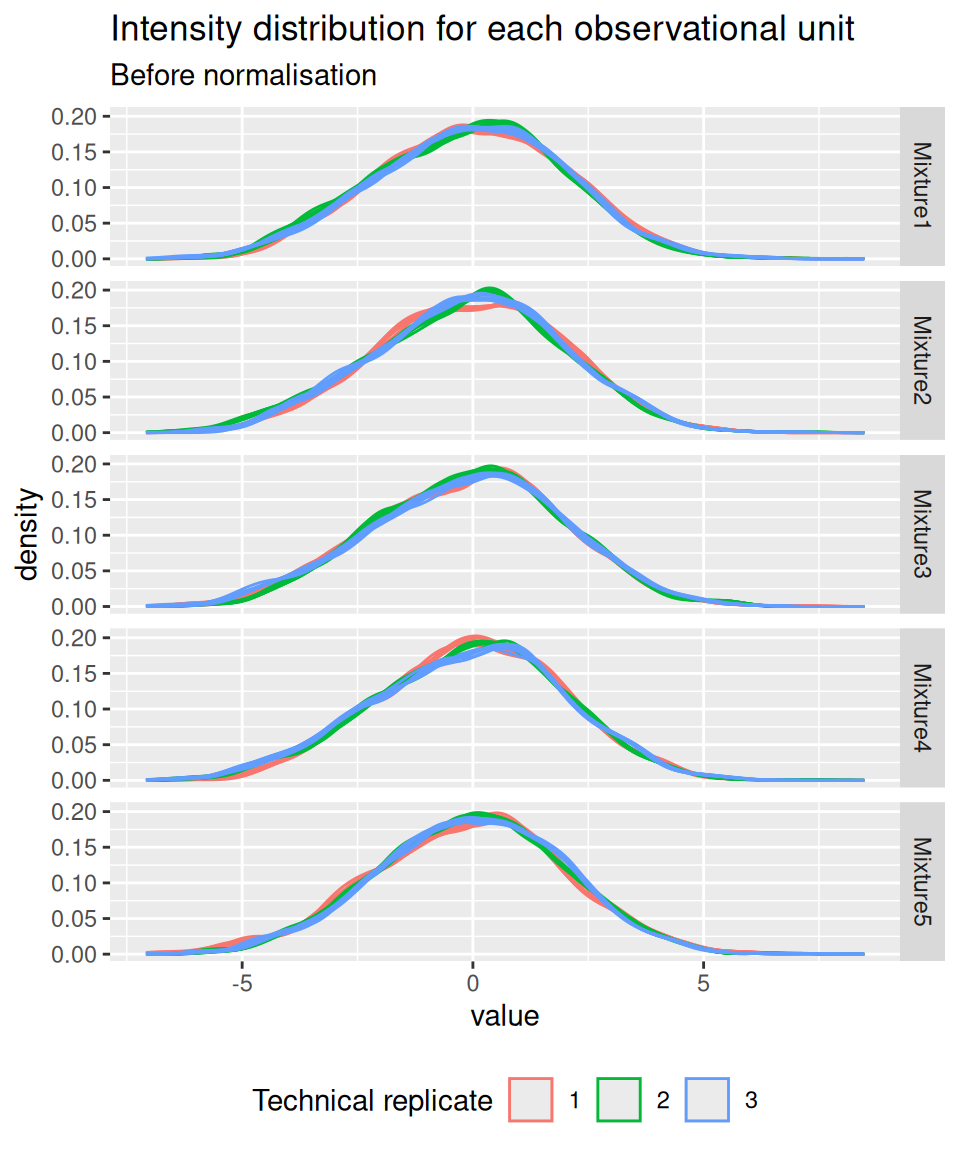

4.6 Summarisation

Below, we illustrate the challenges of summarising TMT data using one of the UPS proteins in Mixture 1 (separating the data for each technical replicate). We also focus on the 0.125x and the 1x spike-in conditions. We illustrate the different peptide ions on the x axis and plot the log2 normalised intensities across samples on y axis. All the points belonging to the same sample are linked through a grey line.

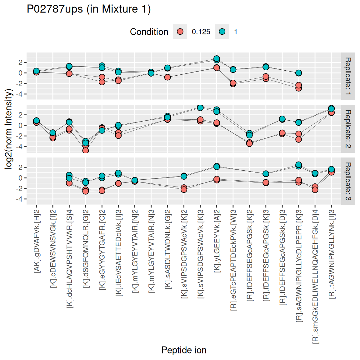
We see that the same challenges observed for LFQ data also apply to TMT data. Briefly:

1. Data for a protein can consist of many peptide ions.
2. Peptide ions have different intensity baselines.
3. There is strong missingness across runs (compare points between replicates), but the missingness is mitigated within runs (compare points within replicates. Note that the data points from one peptide ion in one replicate has been extracted from a single MS2 spectrum.).
4. Subtle intensity shifts for the same peptide across different replicates, called spectrum effects, are caused by small run-to-run fluctuations.
5. Presence of outliers. For instance, the first peptide ion doesn’t show the same change in intensity between conditions compared to majority of the peptides.

Here, we summarise the ion-level data into protein intensities through the median polish approach, which alternately removes the peptide-ions and the sample medians from the data until the summaries stabilise. Removing the peptide-ion medians will solve issue 2. as it removes the ion-specific effects. Using the median instead of the mean will solve issue 5. Note that we perform summarisation for each run separately, hence the ion effect will be different for each run, effectively allowing for a spectrum effect and solving issue 4.

summNames <- paste0(inputNames, "_proteins")
(spikein <- aggregateFeatures(
    spikein, i = normNames,  name = summNames,
    fcol = "Protein.Accessions", fun = MsCoreUtils::medianPolish,
    na.rm = TRUE
))

## An instance of class QFeatures (type: bulk) with 60 sets:
## 
##  [1] Mixture1_01: SummarizedExperiment with 1719 rows and 8 columns 
##  [2] Mixture1_02: SummarizedExperiment with 1722 rows and 8 columns 
##  [3] Mixture1_03: SummarizedExperiment with 1776 rows and 8 columns 
##  ...
##  [58] Mixture5_01_proteins: SummarizedExperiment with 307 rows and 8 columns 
##  [59] Mixture5_02_proteins: SummarizedExperiment with 296 rows and 8 columns 
##  [60] Mixture5_03_proteins: SummarizedExperiment with 299 rows and 8 columns

Up to now, the data from different runs were kept in separate assays. We can now join the normalised sets into an proteins set using joinAssays(). Sets are joined by stacking the columns (samples) in a matrix and rows (features) are matched according to the row names (i.e. the protein identifiers).

spikein <- joinAssays( 
    spikein, summNames, "proteins"
)

5 Data exploration

We perform data exploration using MDS.

library("scater")
se <- getWithColData(spikein, "proteins")
se <- runMDS(as(se, "SingleCellExperiment"), exprs_values = 1)
plotMDS(se, colour_by = "Condition") +
  plotMDS(se, colour_by = "Run") + 
  plotMDS(se, colour_by = "Mixture")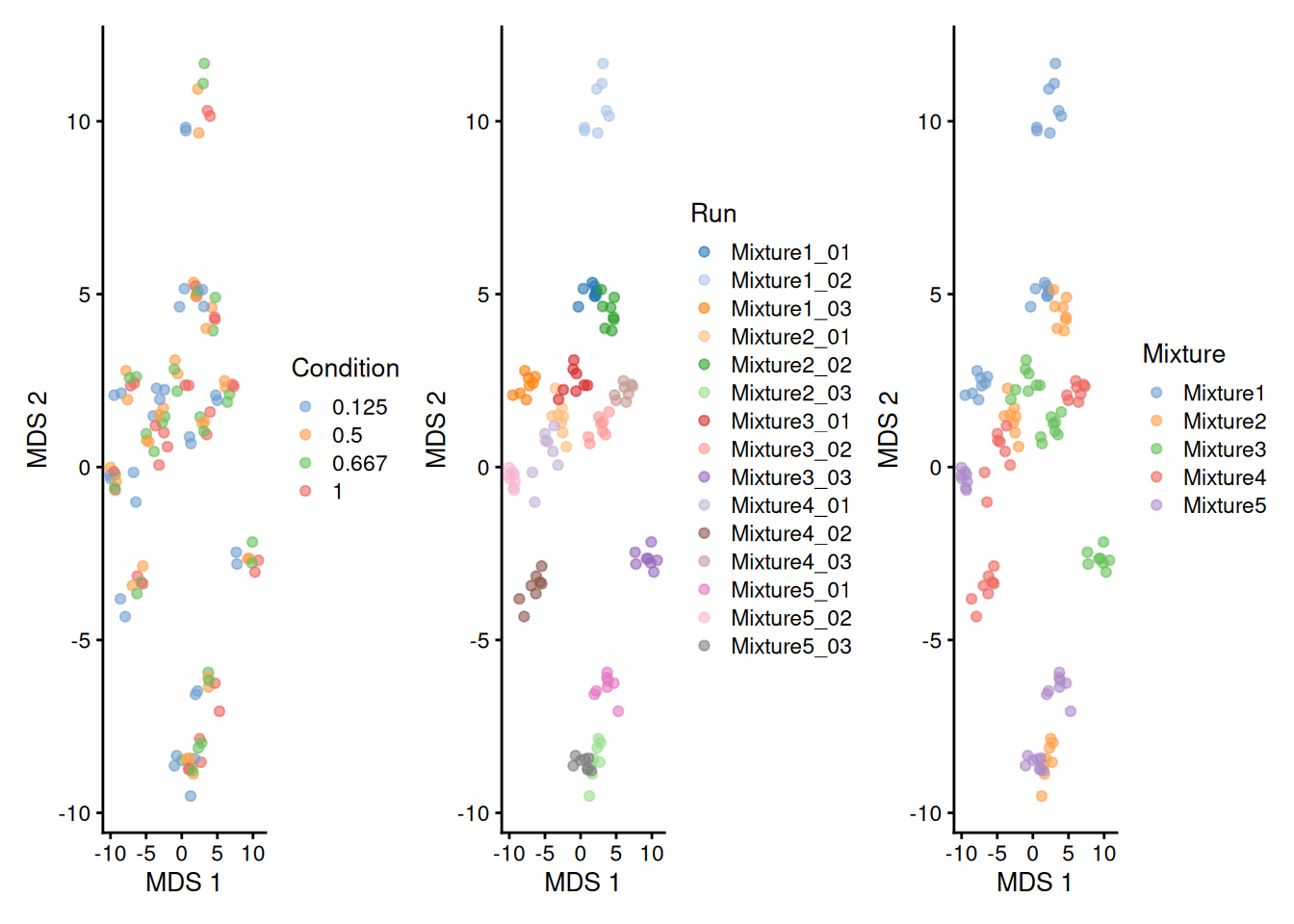

There is a strong run-to-run effect, which is partly explained by a mixture effect as the runs from the same mixture tend to be closer than runs from different mixtures. The condition effect is much more subtle to find, probably because we know only a few UPS proteins were spiked in while the majority of the background proteins are unchanged. We can see that normalisation and summarisation alone are not sufficient to correct for these unwanted effects. We will take care of these effects during the data modelling.

6 Data modelling

Proteomics data contain several sources of variation that need to be accounted for by the model. We will build the model by progressively adding the different sources of variation.

6.1 Effect of treatment of interest

We model the source of variation induced by the experimental treatment of interest as a fixed effect, which we consider non-random, i.e. the treatment effect is assumed to be the same in repeated experiments, but it is unknown and has to be estimated. When modelling a typical label-free experiment at the protein level, the model boils down to a linear model, again we suppress the index for protein:

\[ y_r = \mathbf{x}^T_r \boldsymbol{\beta} + \epsilon_r, \]

with \(y_r\) the \(\log_2\)-normalized protein intensities in run r; \(\mathbf{x}_r\) a vector with the covariate pattern for the sample in run \(r\) encoding the intercept, treatment, potential batch effects and confounders; \(\boldsymbol{\beta}\) the vector of parameters that model the association between the covariates and the outcome; and \(\epsilon_r\) the residuals reflecting variation that is not captured by the fixed effects. Note that \(\mathbf{x}_r\) allows for a flexible parameterization of the treatment beyond a single covariate, i.e. including a 1 for the intercept, continuous and categorical variables as well as their interactions. For all models considered in this work, we assume the residuals to be independent and identically distributed (i.i.d) according to a normal distribution with zero mean and constant variance, i.e. \(\epsilon_{r} \sim N(0,\sigma_\epsilon^2)\), that can differ from protein to protein.

Now we defined a model, we must estimate from the data. Using msqrob(), the model translates into the following code:

spikein <- msqrob(
    spikein,  i = "proteins",
    formula = ~  Condition ## fixed effect for experimental condition
)

This model is however incomplete and relying on its results would lead to incorrect conclusions as we are still missing important source of variation. We did therefore not run the modelling command and will expand the model.

6.2 Effect of TMT label and run

As label-free experiments contain only a single sample per run, run-specific effects will be absorbed in the residuals. However, the data analysis of labeled experiments, e.g. using TMT multiplexing, involving multiple MS runs has to account for run- and label-specific effects, explicitly. If all treatments are present in each run, and if TMT label swaps are performed so as to avoid confounding between label and treatment, then the model parameters can be estimated using fixed label and run effects. Indeed, for these designs run acts as a blocking variable as all treatment effects can be estimated within each run.

However, for more complex designs this is no longer possible and the uncertainty in the estimation of the mean model parameters can involve both within and between TMT label and run variability. For these designs we can resort to mixed models where the label and run effect are modelled using random effects, i.e. they are considered as a random sample from the population of all possible runs and TMT labels, which are assumed to be i.i.d normally distributed with mean 0 and constant variance, \(u_r \sim N(0,\sigma^{2,\text{run}})\) (\(u_{label} \sim N(0,\sigma^{2,\text{label}})\)). The use of random effects thus models the correlation in the data, explicitly. Indeed, protein intensities that are measured within the same run/label will be more similar than protein intensities between runs/labels.

Hence, the model is extended to:

\[ y_{rl} = \mathbf{x}^T_{rl} \boldsymbol{\beta} + u_l^\text{label} + u_r^\text{run} + \epsilon_{rl} \] with \(y_{rl}\) the normalised \(\log_2\) protein intensities in run \(r\) and label \(l\), \(u_l^\text{label}\) the effect introduced by the label \(l\), and \(u_r^\text{run}\) the effect for MS run \(r\).

This translates in the following code:

spikein <- msqrob(
    spikein,  i = "proteins",
    formula = ~  Condition + ## fixed effect for experimental condition
        (1 | Label) + ## random effect for label
        (1 | Run) ## random effect for MS run
    )

This model is still incomplete and is no executed as we still need to account that each mixture has been replicated three times.

6.3 Effect of replication

Some experiments also include technical replication where a TMT mixture can be acquired multiple times. This again will induce correlation. Indeed, protein intensities from the same mixture will be more alike than those of different mixtures. Hence, we also include a random effect to account for this pseudo-replication, i.e. \(u^\text{mix}_m \sim N(0, \sigma^{2,\text{mix}})\). The model thus extends to:

\[ y_{rlm} = \mathbf{x}^T_{rlm} \boldsymbol{\beta} + u_{l}^\text{label} + u_r^\text{run} + u_m^\text{mix} + \epsilon_{rlm} \]

with \(m\) the index for mixture.

The model translates to the following code:

spikein <- msqrob(
    spikein,  i = "proteins",
    formula = ~  Condition + ## fixed effect for experimental condition
        (1 | Label) + ## random effect for label
        (1 | Run) + ## random effect for MS run
        (1 | Mixture) ## random effect for mixture
)

This model provides a sensible representation of the sources of variation in the data.

7 Statistical inference

We can now convert the biological question “does the spike-in condition affect the protein intensities?” into a statistical hypothesis. In other words, we need to define the contrast. We plot an overview of the model parameters.

library("ExploreModelMatrix")
vd <- VisualizeDesign(
    sampleData =  colData(spikein),
    designFormula = ~ Condition,
    textSizeFitted = 4
)
vd$plotlist

## [[1]]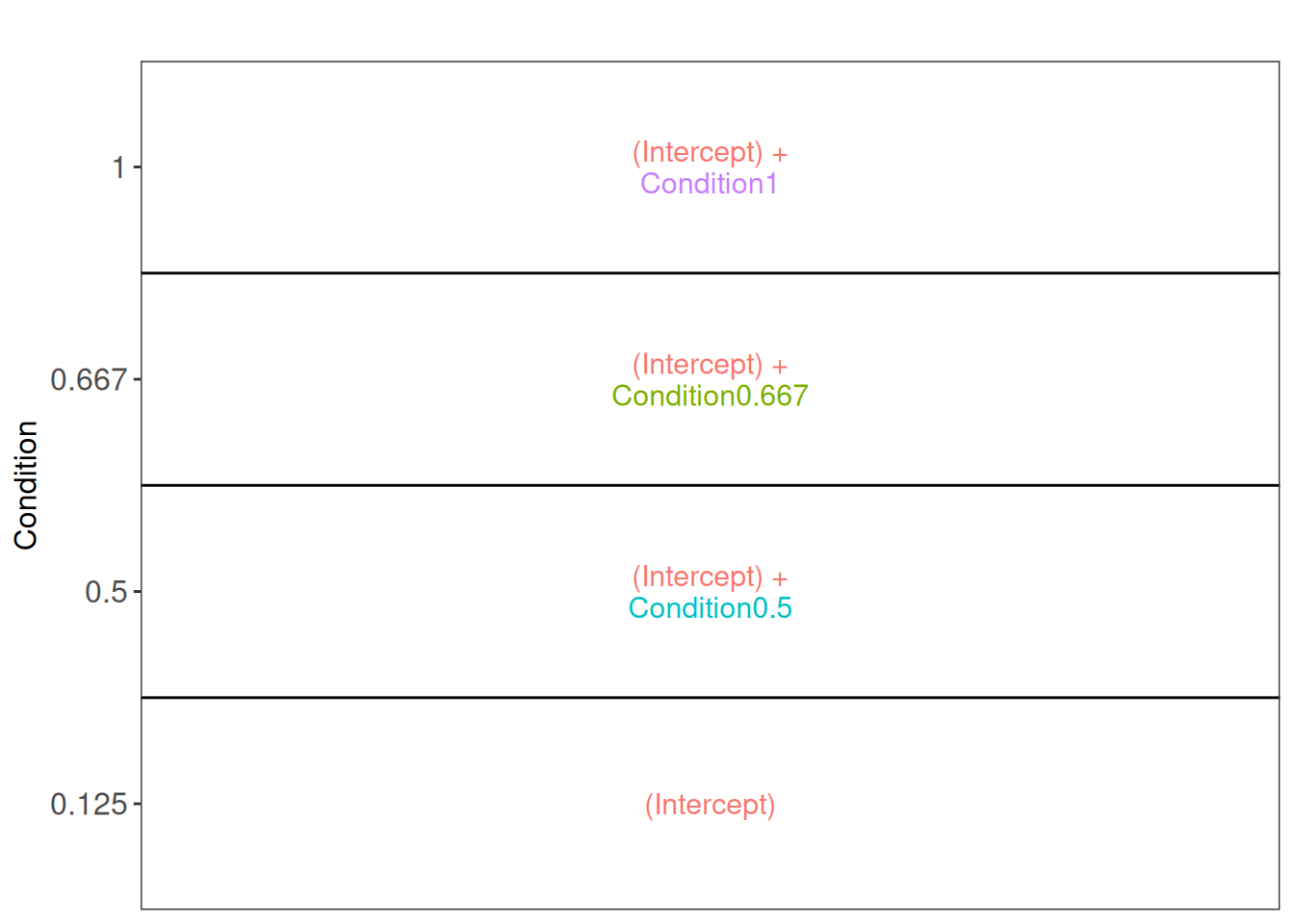

7.1 Hypothesis testing

The average difference intensity between the 1x and the 0.5x conditions is provided by the contrast Condition1 - Condition0.5.

hypothesis <- "Condition1 - Condition0.5 = 0"
L <- makeContrast(
    hypothesis,
    parameterNames = c("Condition1", "Condition0.5")
)

We test our null hypotheses using hypothesisTest() and the estimated model stored in proteins.

spikein <- hypothesisTest(spikein, i = "proteins", contrast = L)
(inference <- rowData(spikein[["proteins"]])[, colnames(L)])

7.2 Volcano plots

We generate a volcano plot with all the results for the 1- 0.5x comparison.

inference$Protein <- rownames(inference)
inference$isUps <- grepl("ups", inference$Protein)
ggplot(inference) +
    aes(x = logFC,
        y = -log10(pval),
        color = isUps) +
    geom_point() +
    geom_hline(yintercept = -log10(inference$pval[which.min(abs(inference$adjPval - 0.05))] )) +
    scale_color_manual(
      values = c("grey20", "firebrick"), name = "",
      labels = c("HeLA background", "UPS standard")
    ) +
    ggtitle("Statistical inference the 1x - 0.5x comparison")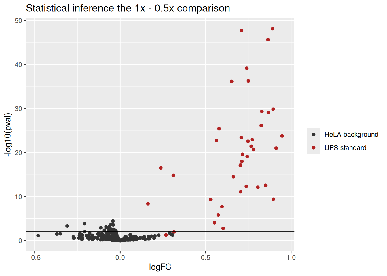 

7.3 Fold change distributions

As this is a spike-in study with known ground truth, we can also plot the log2 fold change distributions against the expected values, in this case 0 for the HeLa proteins and 1 for the UPS standards.

ggplot(inference) +
    aes(y = logFC,
        x = isUps,
        colour = isUps) +
    geom_boxplot() +
    scale_color_manual(
        values = c("grey20", "firebrick"), name = "",
        labels = c("HeLA background", "UPS standard")
    ) +
    ggtitle("Distribution of the log2 fold changes")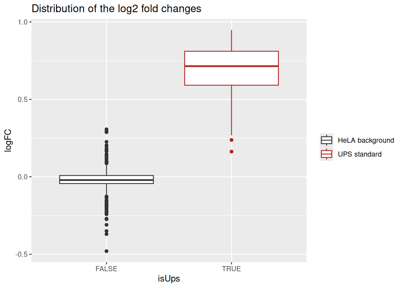

The estimated log2 fold changes for HeLa proteins are closely distributed around 0, as expected. log2 fold changes for UPS standard proteins are distributed toward 1, but it has been underestimated due to ion suppression effects that are characteristic of data set with high spike-in concentrations.

8 Exercise: the mouse diet use case

Let’s repeat this analysis, but on a real-life problem, instead of a synthetic spike-in study.

8.1 Experimental context

The data used in this exercise has been published by Plubell et al. (2017) (PXD005953). The objective of the experiment was to explore the impact of low-fat and high-fat diets on the proteomic content of adipose tissue in mice. It also assesses whether the duration of the diet may impact the results. The authors assigned twenty mice into four groups (5 mice per group) based on their diet, either low-fat (LF) or high-fat (HF), and the duration of the diet, which was classified as short (8 weeks) or long (18 weeks). Samples from the epididymal adipose tissue were extracted from each mice. The samples were then randomly distributed across three TMT 10-plex mixtures for analysis. In each mixture, two reference labels were used, each containing pooled samples that included a range of peptides from all the samples. Not all labels were used, leading to an unbalanced design. Each TMT 10-plex mixture was fractionated into nine parts, resulting in a total of 27 MS runs.

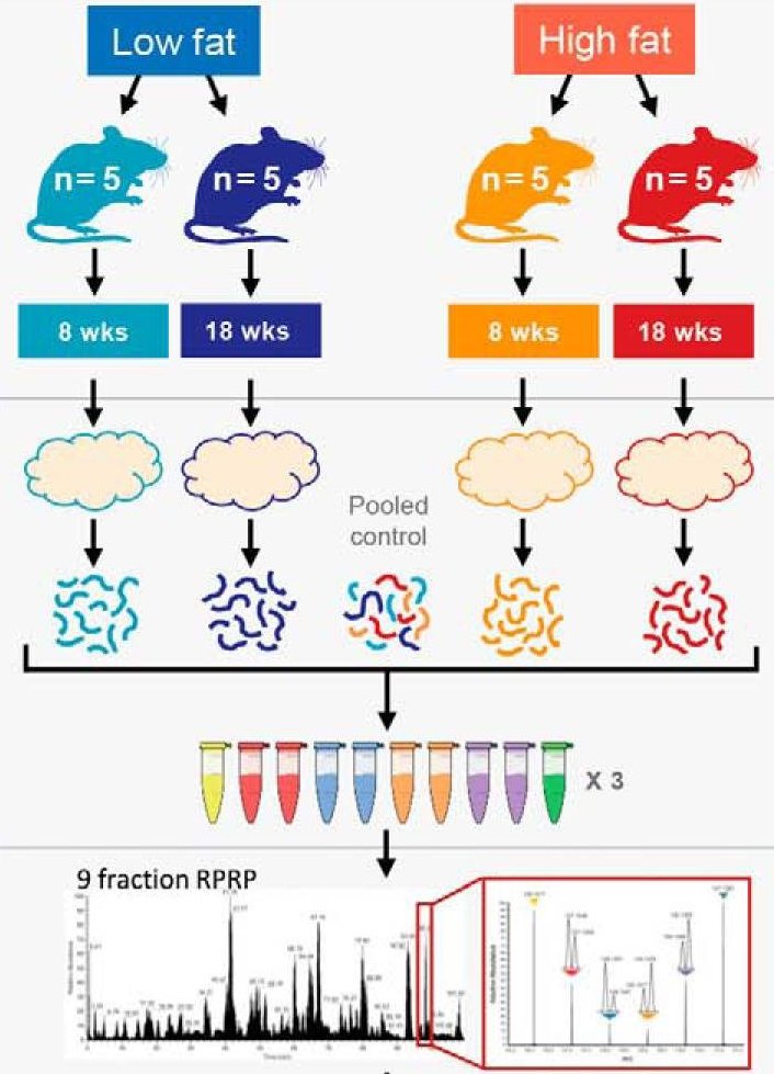
Overview of the experimental design. Taken from Plubell et al. 2017.

8.2 Data

The data were reanalyzed by Huang et al. (2020) and have been deposited in the MSV000084264 MASSiVE repository, but we will retrieve the timestamped data from our Zenodo repository. We need 2 files: the Skyline identification and quantification table generated by the authors and the sample annotation files.

library("BiocFileCache")
bfc <- BiocFileCache()
psmFile <- bfcrpath(bfc, "https://zenodo.org/records/14767905/files/mouse_psms.txt?download=1")
annotFile <- bfcrpath(bfc, "https://zenodo.org/records/14767905/files/mouse_annotations.csv?download=1")

Let’s prepare the data (same approach as above). We will also subset the data set to reduce computational costs. We here randomly sample 500 proteins from the experiment.

## Reading data
psms <- read.delim(psmFile)
coldata <- read.csv(annotFile)
coldata$Duration <- gsub("_.*", "", coldata$Condition) ## 1.
coldata$Diet <- gsub(".*_", "", coldata$Condition) ## 2.
colnames(coldata)[1] <- "Label" ## 3.
## Subsetting data
proteinIds <- unique(psms$Protein.Accessions)
set.seed(1234)
psms <- psms[psms$Protein.Accessions %in% sample(proteinIds, 500), ]
## Converting data
coldata$runCol <- coldata$Run
coldata$quantCols <- paste0("Abundance..", coldata$Label)
mouse <- readQFeatures(psms, colData = coldata,
                       quantCols = unique(coldata$quantCols),
                       runCol = "Spectrum.File", name = "psms")
names(mouse) <- sub("^.*(Mouse.*ACN).*raw", "\\1", names(mouse))

8.3 Data preprocessing

We use a data processing workflow very similar to above.

## Encode missing values
mouse <- zeroIsNA(mouse, names(mouse))
## Sample filtering
mouse <- subsetByColData(
    mouse, mouse$Condition != "Norm" & mouse$Condition != "Long_M"
)
## PSM filtering
mouse <- filterNA(mouse, names(mouse), pNA = 0.7)
mouse <- filterFeatures(
    mouse, ~ Protein.Accessions != "" & ## Remove failed protein inference
        !grepl(";", Protein.Accessions)) ## Remove protein groups
for (i in names(mouse)) {
    rowdata <- rowData(mouse[[i]])
    rowdata$ionID <- paste0(rowdata$Annotated.Sequence, rowdata$Charge)
    rowdata$rowSums <- rowSums(assay(mouse[[i]]), na.rm = TRUE)
    rowdata <- data.frame(rowdata) |>
        group_by(ionID) |>
        mutate(psmRank = rank(-rowSums))
    rowData(mouse[[i]]) <- DataFrame(rowdata)
}
mouse <- filterFeatures(mouse, ~ psmRank == 1)
## Log transformation
sNames <- names(mouse)
mouse <- logTransform(
    mouse, sNames, name = paste0(sNames, "_log"), base = 2
)
## Normalisation
mouse <- normalize(
    mouse, paste0(sNames, "_log"), name = paste0(sNames, "_norm"),
    method = "center.median"
)
## Protein summarisation
mouse <- aggregateFeatures(
    mouse, i = paste0(sNames, "_norm"), name = paste0(sNames, "_proteins"),
    fcol = "Protein.Accessions", fun = MsCoreUtils::medianPolish,
    na.rm=TRUE
)
## Join sets
mouse <- joinAssays(mouse, paste0(sNames, "_proteins"), "proteins")

8.4 Problem statement

Starting from the processed proteins set, build a model accounting for all sources of variation in the experiments (use the figure shown in the experimental context to guide your decisions), and allowing you to answer the following questions:

• What is the difference in protein abundance between low fat and high fat diet after short duration?
• What is the difference in protein abundance between low fat and high fat diet after long duration?
• What is the average difference in protein abundance between low fat and high fat diet?
• Does the diet effect change according to duration? (hint: is there an interaction between diet and duration?)

Note that you should use Diet and Duration as the experimental variables of interest, and you can explore the available variables for modelling using colData(mouse). Recall that you can also explore your data using MDS and colour for the potential sources of variation.

Estimate your model and perform statistical inference using msqrob2. Each question will require you to test a different contrast. Don’t forget that the VisualizeDesign() function can help you with identify the correct combination of parameters to define your contrast.

The report the results using a volcano plot and a differential analysis table to answer the questions.

8.5 Solution

Click to see the solution

Let’s explore the data.

library("scater")
se <- getWithColData(mouse, "proteins") |> 
  as("SingleCellExperiment") |> 
  runMDS(exprs_values = 1)

We plot the MDS and colour each sample based on different potential sources of variation.

plotMDS(se, colour_by = "Run") + ggtitle("Coloured by Run") +
  scale_colour_manual(values = rainbow(27)) +
  plotMDS(se, colour_by = "Fraction") + ggtitle("Coloured by Fraction") +
  plotMDS(se, colour_by = "BioReplicate") + ggtitle("Coloured by BioReplicate") +
  plotMDS(se, colour_by = "Mixture") + ggtitle("Coloured by Mixture") +
  plotMDS(se, colour_by = "Diet") + ggtitle("Coloured by Diet") +
  plotMDS(se, colour_by = "Duration") + ggtitle("Coloured by Duration") &
  theme(legend.position = "none")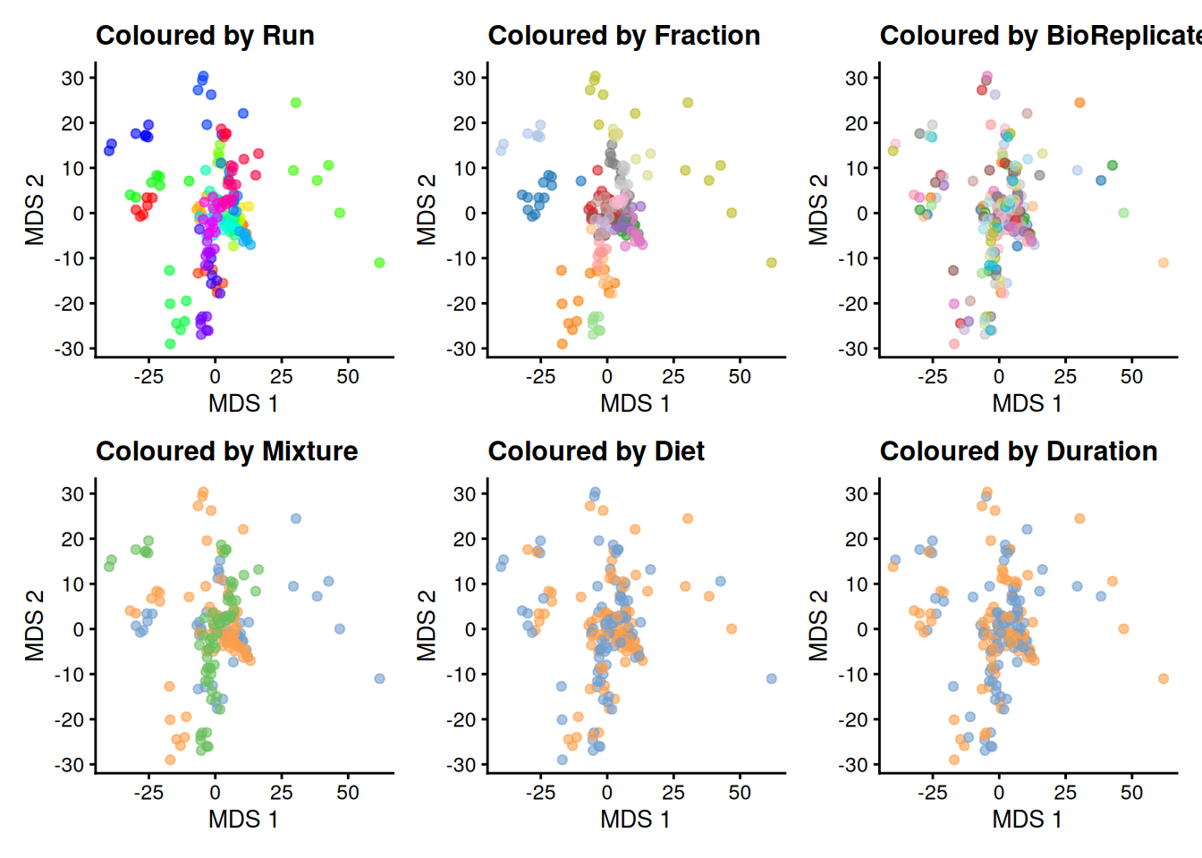 

The data exploration leads to several observations:

• The strongest source of variation is associated with the MS acquisition run.
• Part of this run effect is influenced by which fraction it contains since samples from the same fraction tend to be closer than samples from different fractions.
• It is difficult to identify an effect of mouse (biological replicate) because every run contains distinct mice. However, this does not exclude an effect of mice which has been identified as a potential source of variation and hence should still be modelled.
• There is potentially also an effect of TMT mixture since samples from the same mixtures tend to cluster together (in the center of the plot). However, this effect are more subtle to detect and difficult to disentangle from the run and fraction effects.
• Although again very subtle, we can see within each run that samples from the mice with the same diet tends to group together. However, these effects are overwhelmed by the run effects. An effect of duration is to subtle to pinpoint from the current data exploration.

Data modelling disentangles the different sources of variation, given they are properly defined in the model.

Proteomics data contain several sources of variation that need to be accounted for by the model:

1. Treatment of interest: we model the source of variation induced by the experimental treatment of interest as a fixed effect. Fixed effects are effect that are considered non-random, i.e. the treatment effect is assumed to be the same and reproducible across repeated experiments, but it is unknown and has to be estimated. We will include Diet as a fixed effect that models the fact that a change in diet type can induce changes in protein abundance. Similarly, we also include Duration as a fixed effect to model the change in protein abundance induces by the diet duration. Finally, we will also include an interaction between the two variables allowing that the changes in protein abundance induced by diet type can be different whether the mice were fed for a short or long duration.

2. Biological replicate effect: the experiment involves biological replication as the adipose tissue extracts were sampled from 20 mice (5 mice per Diet x Duration combination). Replicate-specific effects occurs due to uncontrollable factors, such as social behavior, feeding behavior, physical activity, occasional injury,… Two mice will never provide exactly the same sample material, even were they genetically identical and manipulated identically. These effects are typically modelled as random effects which are considered as a random sample from the population of all possible mice and are assumed to be i.i.d normally distributed with mean 0 and constant variance, \(u_{mouse} \sim N(0,\sigma^{2,\text{mouse}})\). The use of random effects thus models the correlation in the data, explicitly. We expect that intensities from the same mouse are more alike than intensities between mice.

length(unique(mouse$BioReplicate))

## [1] 20

3. Labelling effects: the 20 mouse adipose tissue samples have been labelled using 18-plex TMT. We can expect that samples measured within the same TMT label may be more similar than samples measured within different TMT labels. Since these effects may not be reproducible from one experiment to another, for instance because each TMT kit may potentially contain different impurity ratios, we can account for this correlation using a random effect for TMT label.

length(unique(mouse$Label))

## [1] 10

4. Mixture effects: the 20 mouse samples were assigned to one out of 3 mixtures. Again, we expect protein intensities from the same mixture will be more alike than those of different mixtures. Hence, we will add a random effect for mixture.

table(mouse$Mixture)

## 
##  PAMI-176_Mouse_A-J  PAMI-176_Mouse_K-T PAMI-194_Mouse_U-Dd 
##                  54                  63                  63

5. Run effects: protein intensities that are measured within the same run will be more similar than protein intensities between runs. We will use a random effect for run to explicitly model this correlation in the data. Note that each sample has been acquired in 9 fractions, each fraction being measured in a separate run. Accounting for the effects of run will also absorb the effects of fraction.

length(unique(mouse$Run))

## [1] 27

We will model the main effects for Diet and Duration, and a Diet:Duration interaction, to account for proteins for which the Diet effect changes according to Duration, and vice versa, which can be written as Diet + Duration + Diet:Duration, shortened into Diet * Duration (recall the heart example in a previous course). Adding the technical sources of variation, the model becomes.

model <- ~ Diet * Duration + ## (1) fixed effect for Diet and Duration with interaction
  (1 | BioReplicate) +  ## (2) random effect for biological replicate (mouse)      
  (1 | Label) + ## (3) random effect for label
  (1 | Mixture) + ## (4) random effect for mixture
  (1 | Run) ## (5) random effect for MS run

We estimate the model with msqrob().

mouse <- msqrob(mouse, i = "proteins", formula = model)

Difference between low fat and high fat diet after short duration

We need to convert this question in a combination of the model parameters. We guide the contrast definition using the ExploreModelMatrix package. Since we are not interested in technical effects, we will only focus on the variables of interest, here Diet * Duration.

library("ExploreModelMatrix")
vd <- VisualizeDesign(
    sampleData =  colData(mouse),
    designFormula = ~ Diet * Duration,
    textSizeFitted = 4
)
vd$plotlist[[1]]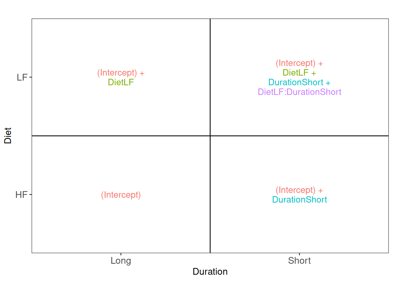

Assessing the difference between low-fat and high-fat diets for short duration boils down to assessing the difference between the Short_LF and Short_HF. The mean for the short low-fat diet group is defined by (Intercept) + DietLF + DurationShort + DietLF:DurationShort. The mean for the short high-fat diet group is defined by (Intercept) + DurationShort. The difference between the two results in the contrast below:

(L <- makeContrast(
    "DietLF + DietLF:DurationShort = 0",
    parameterNames = c("DietLF", "DietLF:DurationShort")
))

##                      DietLF + DietLF:DurationShort
## DietLF                                           1
## DietLF:DurationShort                             1

mouse <- hypothesisTest(mouse, i = "proteins", L)

Let us retrieve the result table from the rowData. Note that the model column is named after the column names of the contrast matrix L.

inference <- rowData(mouse[["proteins"]])[[colnames(L)]]
head(inference, 10)

The table contains the hypothesis testing results for every protein.

We can use the table above directly to build a volcano plot using ggplot2 functionality.

ggplot(inference) +
    aes(x = logFC, y = -log10(pval)) +
    geom_hline(yintercept = -log10(inference$pval[which.min(abs(inference$adjPval - 0.05))] )) +
    geom_point() +
    ggtitle("Statistical inference on differences between LF and HF (short duration)",
            paste("Hypothesis test:", colnames(L), "= 0"))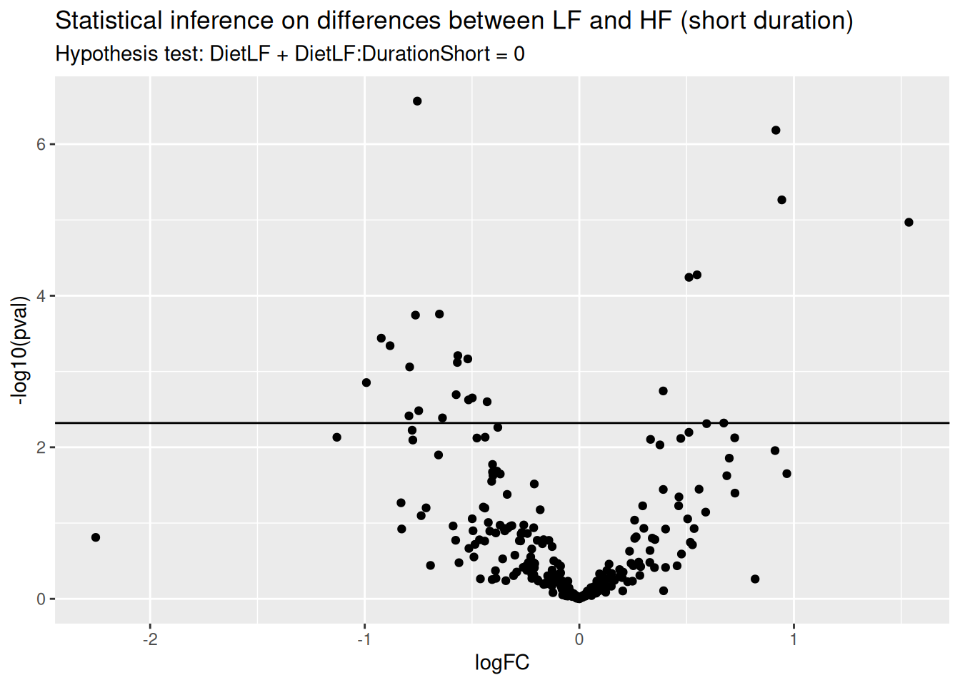

In this example (remember this is a subset of the complete data set), only a few proteins pass the significance threshold of 5% FDR.

Difference between low fat and high fat diet after long duration

Following the same approach as above, the hypothesis test becomes:

L <- makeContrast("DietLF = 0", parameterNames = "DietLF")
mouse <- hypothesisTest(mouse, i = "proteins", L)
inference <- rowData(mouse[["proteins"]])[[colnames(L)]]
head(inference)

And we plot the results.

ggplot(inference) +
    aes(x = logFC, y = -log10(pval)) +
    geom_hline(yintercept = -log10(inference$pval[which.min(abs(inference$adjPval - 0.05))] )) +
    geom_point() +
    ggtitle("Statistical inference on differences between LF and HF (long duration)",
            paste("Hypothesis test:", colnames(L), "= 0"))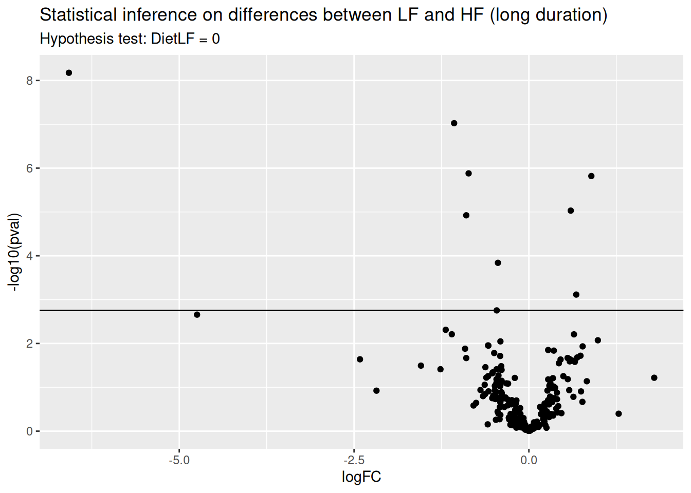

Again, only a few proteins come out differentially abundant between the two diets, but after a long diet duration.

Average difference between low fat and high fat diet

One may want to identify the set of proteins that are systematically differentially abundant between diets, irrespective of the duration. To answer this question, we want to infer on the average difference between group LF and group HF. The average low-fat diet is defined by ((Intercept) + DietLF + DurationShort + DietLF:DurationShort + (Intercept) + DietLF)/2. The average high-fat diet group is defined by ((Intercept) + DurationShort + (Intercept))/2. The difference between the two results in the hypothesis test below:

L <- makeContrast(
    "DietLF + (DietLF:DurationShort)/2 = 0",
    parameterNames = c("DietLF", "DietLF:DurationShort")
)
mouse <- hypothesisTest(mouse, i = "proteins", L)
(inference <- rowData(mouse[["proteins"]])[[colnames(L)]])

And we plot the results.

ggplot(inference) +
    aes(x = logFC, y = -log10(pval)) +
    geom_hline(yintercept = -log10(inference$pval[which.min(abs(inference$adjPval - 0.05))] )) +
    geom_point() +
    ggtitle("Statistical inference on average difference between LF and HF",
            paste("Hypothesis test:", colnames(L), "= 0"))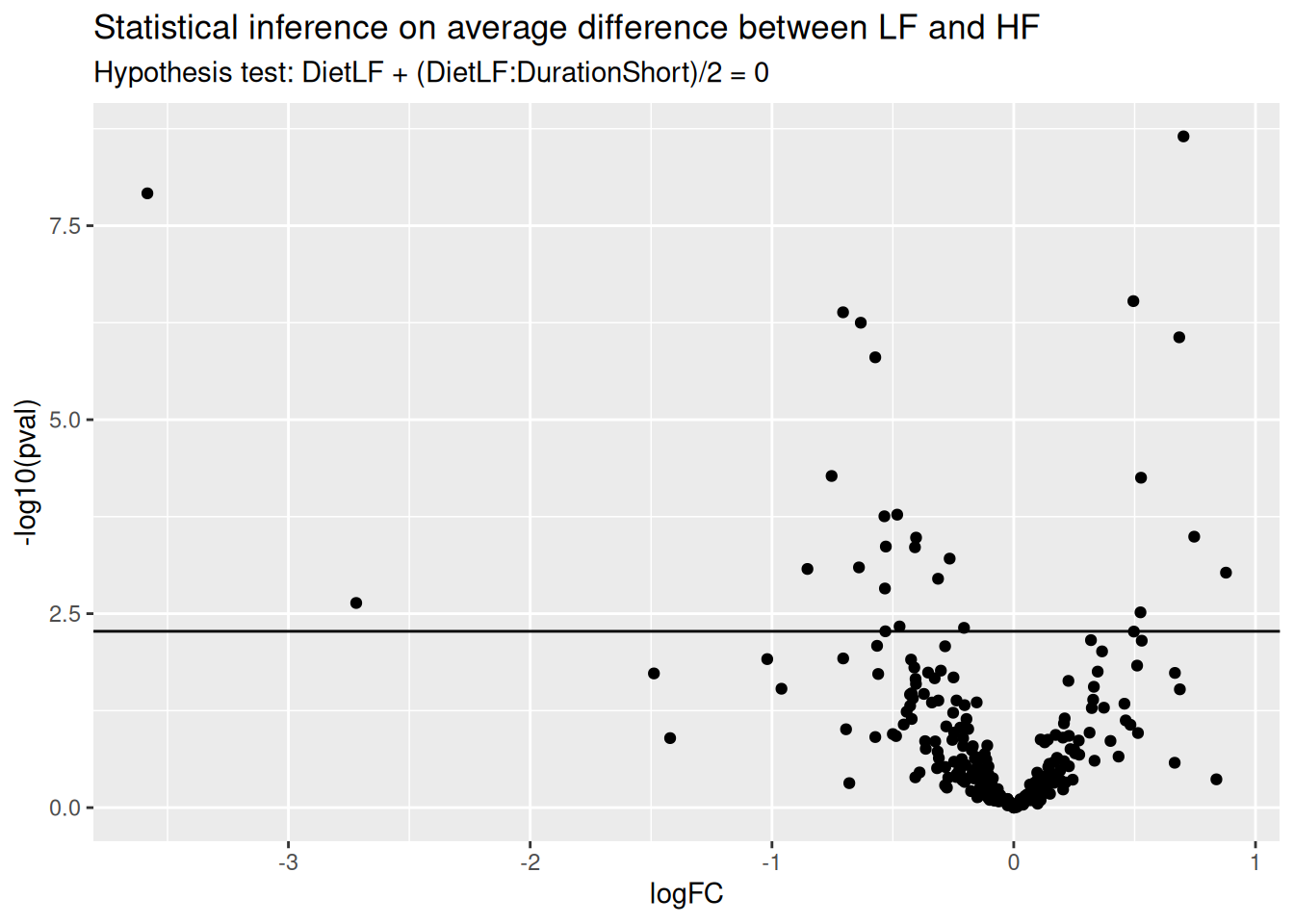

Interaction: does the diet effect change according to duration?

We will now explore whether the effect of diet on protein abundance may be affected by duration, i.e. we want to infer on the difference of differences. The difference between hypothesis 1 and 2 is (DietLF + DietLF:DurationShort) - (DietLF) and results in the hypothesis below:

We can proceed with the same statistical pipeline.

L <- makeContrast(
    "DietLF:DurationShort = 0",
    parameterNames = "DietLF:DurationShort"
)
mouse <- hypothesisTest(mouse, i = "proteins", L)
(inference <- rowData(mouse[["proteins"]])[[colnames(L)]])

And we plot the results.

ggplot(inference) +
    aes(x = logFC, y = -log10(pval)) +
    geom_hline(yintercept = -log10(inference$pval[which.min(abs(inference$adjPval - 0.05))] )) +
    geom_point() +
    ggtitle("Statistical inference on the effect of duration on the differences between diets",
            paste("Hypothesis test:", colnames(L), "= 0"))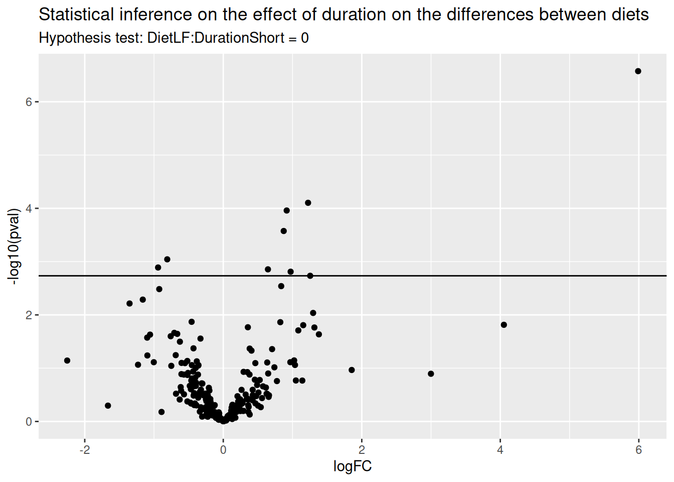

9 Session Info

With respect to reproducibility, it is highly recommended to include a session info in your script so that readers of your output can see your particular setup of R.

sessionInfo()

## R version 4.5.1 (2025-06-13)
## Platform: x86_64-pc-linux-gnu
## Running under: Ubuntu 24.04.3 LTS
## 
## Matrix products: default
## BLAS:   /usr/lib/x86_64-linux-gnu/blas/libblas.so.3.12.0 
## LAPACK: /usr/lib/x86_64-linux-gnu/lapack/liblapack.so.3.12.0  LAPACK version 3.12.0
## 
## locale:
##  [1] LC_CTYPE=en_US.UTF-8       LC_NUMERIC=C              
##  [3] LC_TIME=en_US.UTF-8        LC_COLLATE=en_US.UTF-8    
##  [5] LC_MONETARY=en_US.UTF-8    LC_MESSAGES=en_US.UTF-8   
##  [7] LC_PAPER=en_US.UTF-8       LC_NAME=C                 
##  [9] LC_ADDRESS=C               LC_TELEPHONE=C            
## [11] LC_MEASUREMENT=en_US.UTF-8 LC_IDENTIFICATION=C       
## 
## time zone: Europe/Brussels
## tzcode source: system (glibc)
## 
## attached base packages:
## [1] stats4    stats     graphics  grDevices utils     datasets  methods  
## [8] base     
## 
## other attached packages:
##  [1] ExploreModelMatrix_1.21.0   scater_1.37.0              
##  [3] scuttle_1.19.0              SingleCellExperiment_1.31.0
##  [5] BiocFileCache_2.99.0        dbplyr_2.5.0               
##  [7] BiocParallel_1.43.0         patchwork_1.3.0            
##  [9] ggplot2_3.5.2               dplyr_1.1.4                
## [11] msqrob2_1.17.1              QFeatures_1.19.3           
## [13] MultiAssayExperiment_1.35.1 SummarizedExperiment_1.39.0
## [15] Biobase_2.69.0              GenomicRanges_1.61.0       
## [17] GenomeInfoDb_1.45.3         IRanges_2.43.0             
## [19] S4Vectors_0.47.0            BiocGenerics_0.55.0        
## [21] generics_0.1.3              MatrixGenerics_1.21.0      
## [23] matrixStats_1.5.0          
## 
## loaded via a namespace (and not attached):
##   [1] RColorBrewer_1.1-3      rstudioapi_0.17.1       jsonlite_2.0.0         
##   [4] magrittr_2.0.3          ggbeeswarm_0.7.2        farver_2.1.2           
##   [7] nloptr_2.2.1            rmarkdown_2.29          vctrs_0.6.5            
##  [10] memoise_2.0.1           minqa_1.2.8             htmltools_0.5.8.1      
##  [13] S4Arrays_1.9.0          BiocBaseUtils_1.11.0    curl_6.2.2             
##  [16] BiocNeighbors_2.3.0     SparseArray_1.9.0       sass_0.4.10            
##  [19] bslib_0.9.0             htmlwidgets_1.6.4       plyr_1.8.9             
##  [22] httr2_1.1.2             cachem_1.1.0            igraph_2.1.4           
##  [25] mime_0.13               lifecycle_1.0.4         pkgconfig_2.0.3        
##  [28] rsvd_1.0.5              Matrix_1.7-4            R6_2.6.1               
##  [31] fastmap_1.2.0           rbibutils_2.3           shiny_1.10.0           
##  [34] clue_0.3-66             digest_0.6.37           irlba_2.3.5.1          
##  [37] RSQLite_2.3.11          beachmat_2.25.0         filelock_1.0.3         
##  [40] labeling_0.4.3          httr_1.4.7              abind_1.4-8            
##  [43] compiler_4.5.1          bit64_4.6.0-1           withr_3.0.2            
##  [46] viridis_0.6.5           DBI_1.2.3               MASS_7.3-65            
##  [49] rappdirs_0.3.3          DelayedArray_0.35.1     tools_4.5.1            
##  [52] vipor_0.4.7             beeswarm_0.4.0          httpuv_1.6.16          
##  [55] glue_1.8.0              nlme_3.1-168            promises_1.3.2         
##  [58] grid_4.5.1              cluster_2.1.8.1         reshape2_1.4.4         
##  [61] gtable_0.3.6            tidyr_1.3.1             BiocSingular_1.25.0    
##  [64] ScaledMatrix_1.17.0     XVector_0.49.0          ggrepel_0.9.6          
##  [67] pillar_1.10.2           stringr_1.5.1           limma_3.65.0           
##  [70] later_1.4.2             rintrojs_0.3.4          splines_4.5.1          
##  [73] lattice_0.22-7          bit_4.6.0               tidyselect_1.2.1       
##  [76] knitr_1.50              reformulas_0.4.1        gridExtra_2.3          
##  [79] ProtGenerics_1.41.0     shinydashboard_0.7.3    xfun_0.52              
##  [82] statmod_1.5.0           DT_0.33                 stringi_1.8.7          
##  [85] UCSC.utils_1.5.0        lazyeval_0.2.2          yaml_2.3.10            
##  [88] boot_1.3-31             evaluate_1.0.3          codetools_0.2-20       
##  [91] MsCoreUtils_1.21.0      tibble_3.2.1            cli_3.6.5              
##  [94] xtable_1.8-4            Rdpack_2.6.4            jquerylib_0.1.4        
##  [97] Rcpp_1.0.14             png_0.1-8               parallel_4.5.1         
## [100] blob_1.2.4              AnnotationFilter_1.33.0 lme4_1.1-37            
## [103] viridisLite_0.4.2       scales_1.4.0            purrr_1.0.4            
## [106] crayon_1.5.3            rlang_1.1.6             cowplot_1.1.3          
## [109] shinyjs_2.1.0

References

Huang, Ting, Meena Choi, Manuel Tzouros, Sabrina Golling, Nikhil Janak Pandya, Balazs Banfai, Tom Dunkley, and Olga Vitek. 2020. “MSstatsTMT: Statistical Detection of Differentially Abundant Proteins in Experiments with Isobaric Labeling and Multiple Mixtures.” Mol. Cell. Proteomics 19 (10): 1706–23.

Plubell, Deanna L, Phillip A Wilmarth, Yuqi Zhao, Alexandra M Fenton, Jessica Minnier, Ashok P Reddy, John Klimek, Xia Yang, Larry L David, and Nathalie Pamir. 2017. “Extended Multiplexing of Tandem Mass Tags (TMT) Labeling Reveals Age and High Fat Diet Specific Proteome Changes in Mouse Epididymal Adipose Tissue.” Mol. Cell. Proteomics 16 (5): 873–90.