Lab 6: Large Scale Inference

High Dimensional Data Analysis practicals

Change log

---

## install packages with:
# if (!requireNamespace("remotes", quietly = TRUE)) {
#     install.packages("remotes")
# }
# remotes::install_github("statOmics/HDDAData")

library(HDDAData)

1 Introduction

In this lab session we will look at the following topics

• FWER
• FDR
• Multiple testing problem in a real dataset

1.1 Testing many hypotheses

To demonstrate the ideas we will be working with, we will simulate artificial data. Note that since we are doing simulations, we can control everything and also know exactly what the underlying “true” distribution is (sometimes also called the “ground truth”). However, keep in mind that this is an unlikely representation of real-world data.

In particular, we will simulate data for multiple hypothesis tests where the null hypothesis is always true. This means that for the $i$-th test, if we let $\mu_{1i}$ and $\mu_{2i}$ represent the means of the two populations of interest, the null hypothesis for comparing the two means is $H_{0i} : \mu_{1i} = \mu_{2i}$. Let the alternative hypothesis of this test be $H_{1i} : \mu_{1i} \neq \mu_{2i}$, i.e., we perform a two-tailed test. Suppose we have data collected from both populations, given by $X_{1i}$ and $X_{2i}$ of size $n_{1i}$ and $n_{2i}$, respectively, and assume that both populations have the same known variance $\sigma_i^2$. Then we can test this hypothesis by using a Z-test statistic, given by

$$Z_i=\frac{\bar X_{1i}-\bar X_{2i}}{\sigma_i\sqrt{1/n_{1i}+1/n_{2i}}} \, .$$

Under the null hypothesis, the scores will be distributed as a standard normal $Z_i\sim N(0,1)$. The null hypothesis is rejected in favor of the alternative if $z_i < \phi_{\alpha_i/2}$ or $z_i > \phi_{1-\alpha_i/2}$, or equivalently if $|z_i| > \phi_{1-\alpha_i/2}$, where $\phi_{\alpha_i/2}$ is the $\alpha_i/2$th quantile of the standard normal distribution.

In a multiple hypothesis testing setting, we will perform $m$ tests using the same test statistic. If the null were true for all hypotheses, we would end up with a sample $z_1,\ldots,z_m$ from a standard normal distribution.

In this setting, we can only make one type of error: wrongly rejecting the null hypothesis, i.e. a type 1 error. The probability of making this error is given by

$$\alpha_i=\text{P}\{\text{ reject } H_{0i} | H_{0i}\}$$

(the $| H_{0i}$ part should be read as “given that the null hypothesis is true”).

If we now perform $m_0$ such tests (using the 0 subscript to denote that they are all hypotheses for which the null is true), we can summarise the possible outcomes as in the table below:

	Accept H_0	Reject H_0	Total
H_0 True	U (True Negative)	V (False Positive)	m_0

Here, $U$ and $V$ represent the total number of true negative and false positive results we get, respectively, out of $m_0$ total tests.

As an example, let’s simulate the scenario above. In the code below, the replicate function is used to repeat the same procedure a number of times. Essentially, the following steps are performed :

1. Sample $N = 50$ observations for 2 hypothetical groups from normal distributions with the same mean and known variance.
2. Calculate Z-test statistics based on the 2 group means.
3. Repeat steps 1 to 2 m0 times.

This mimics performing m0 hypothesis tests on data for which we know the null hypothesis is true.

# Set parameters for the simulation
N <- 50 # samples per group
m0 <- 1000 # number of hypothesis tests
mu_1 <- 3 # true mean group 1
mu_2 <- 3 # true mean group 2
sigma <- 1 # known variance
denom <- sigma * sqrt(2 / N) # denominator for Z-scores

set.seed(987654321) # seed for reproducibility
z_stats <- replicate(m0, {
  group1 <- rnorm(N, mean = mu_1, sd = sqrt(sigma))
  group2 <- rnorm(N, mean = mu_2, sd = sqrt(sigma))

  # Calculate Z-test statistic
  (mean(group2) - mean(group1)) / denom
})

# Visualize Z-test statistics
hist(z_stats, breaks = 50, freq = FALSE, main = "Z-test statistics under H_0")
# Overlay theoretical standard normal
lines(x <- seq(-5, 5, length.out = 100), dnorm(x), col = "dodgerblue", lwd = 3)
# Draw vertical lines at 2.5 and 97.5th percentiles
abline(v = qnorm(c(0.025, 0.975)), col = "firebrick", lty = 2, lwd = 3)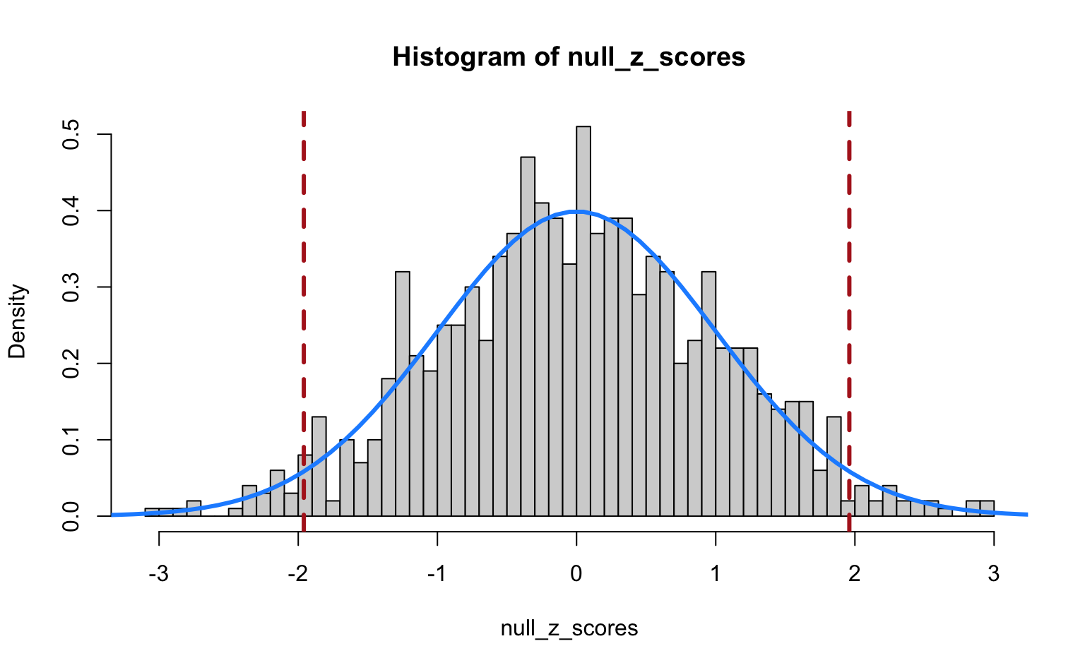

We see that the Z-test statistics nicely follow a standard normal distribution. The vertical dashed lines indicate the 2.5th and 97.5th percentiles of the standard normal. The regions outside these lines indicate the Z-scores that we would call significant if we used a cut-off of $\alpha = 0.05$ for a two-tailed test. So, even though we simulated data under the null hypothesis, our Z-test still returns “significant” results for a number of cases just by chance!

Let’s calculate the p-values for our hypothesis tests and see what the damage is. To calculate the p-values, we use the pnorm() function in this case, which returns the value of the standard normal CDF (i.e. pnorm(x) = $P(Z < x)$). Since we consider a two-tailed test, we take the absolute values of the Z-scores and set the lower.tail argument in pnorm to FALSE (by default it’s TRUE), so that we get pnorm(abs(x), lower.tail = FALSE) = $P(Z > |x|)$ and multiply this value by 2.

null_pvals <- 2 * pnorm(abs(z_stats), lower.tail = FALSE)
alpha <- 0.05

hist(null_pvals, breaks = seq(0, 1, by = 0.05))
abline(v = alpha, col = "firebrick", lwd = 3)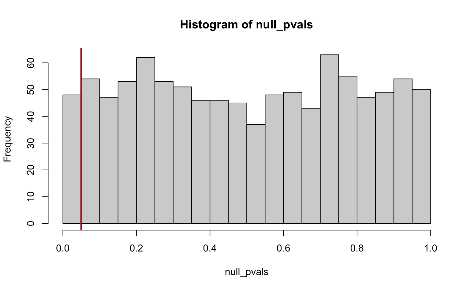

called <- (null_pvals < alpha)

# V = number of false positives, in this case: all significant tests
(V <- sum(called))
#> [1] 51
mean(called) # V / m0
#> [1] 0.051

So we get 51 significant tests (false positives) out of a total of 1000, which is, unsurprisingly, approximately equal to our significance cutoff $\alpha$. Note also that the p-values are uniformly distibuted under the null hypothesis by definition.

If we had carried out only a few tests (say 10) it would be very unlikely to observe a false positive (on average: 0.05 * 10 = 0.5 false positives) at $\alpha = 0.05$, but since now we’re carrying out so many, we’re almost guaranteed to get false positives. This is what is known as the multiple hypothesis testing problem.

Note that in real-world data the quantities $U$ and $V$ are unknown (because we don’t know the truth; if we did, we wouldn’t have to carry out any hypothesis tests in the first place). However, by using simulated data, we do know the truth and so we can explore these quantities.

1.2 The family-wise error rate

If we carry out many tests, we’re almost guaranteed to get type I errors, just by chance. Therefore the type I error rate is no longer a relevant metric. Instead, we consider the Familywise Error Rate (FWER), given by

$$\text{FWER}=\text{P}\{V > 0\} = \text{P}\{\text{rejecting at least one } H_{0i}| H_0\}$$

where $H_0$ is the intersection of all partial nulls ($H_{0i}$) $i=1,\ldots,m_0$. In general, we would prefer testing procedures that keep the FWER under control, i.e. correct for the multiplicity problem. So instead of choosing $\alpha$ to control the probability of getting a false positive in each test, we try to control the FWER, i.e. the probability of getting at least one false positive in our set of hypothesis tests.

In the following exercises, we will explore this idea on some synthetic data. We will simulate performing hypothesis tests for which the null distribution is always true for different values of m0.

To simplify the code, we will directly sample the Z-test statistics from a standard normal (instead of sampling the individual groups and then performing the test on them, as shown above). We can also skip the p-value calculation and compare our Z-test statistics directly to the $(1 - \alpha) / 2$th quantile of the standard normal distribution (using the qnorm() function).

Tasks

1. Set m0 = 5 and generate m0 Z-test statistics by sampling from the standard normal distribution. Check which ones are significant using a cutoff alpha = 0.05

2. Calculate $V$, the number of significant tests.

3. Check whether V > 0 (at least one significant) and store the result in a variable.

4. Repeat steps 1-3 1000 times and keep track of the result in step 3 by storing it in a vector.

5. Now compute the FWER as the proportion of times $V$ was greater than 0.

6. Repeat the same procedure for m0 = 50 and m0 = 1000. Interpret the results.

Solution

To avoid repeated code, the simulations over the different values of m_0 are combined into one code block.

# Repeat 1000 times for m0 = 5, 50 and 1000
set.seed(987654321)
B <- 1000 # number of simulations
m0_vec <- c(5, 50, 1000)
alpha <- 0.05
# Initialize empty vector to store FWER results
fwer <- numeric(length = length(m0_vec))
names(fwer) <- paste("m0 =", m0_vec)

# Loop over m0 values and simulate test statistics
for (i in seq_along(m0_vec)) {
  # Simulate B times, each time recording V > 0
  at_least_one_signif <- replicate(B, {
    null_stats <- rnorm(m0_vec[i], mean = 0, sd = 1) # simulate z-test
    significant_tests <- abs(null_stats) > qnorm(1 - alpha / 2)
    sum(significant_tests) > 0
  })
  fwer[i] <- mean(at_least_one_signif) # proportion of V >= 1
}
fwer
#>    m0 = 5   m0 = 50 m0 = 1000 
#>     0.235     0.925     1.000

2 Controlling the FWER

We saw in the previous exercises that when conducting a large number of hypothesis tests the FWER becomes unacceptably large. So what can we do to lower it? The most straightforward way would be to just lower $\alpha$ (so we get less false positives).

Under the null hypothesis (so the p-values are uniformly distributed), we can write the FWER for $m$ independent tests as

$$\begin{align} \text{FWER} = P(\text{at least one rejection}) &= 1 - P(\text{no rejections}) \\ &= 1 - \prod_{i=1}^{m} P(p_i > \alpha) \\ &= 1 - \prod_{i=1}^{m} (1 - \alpha) \\ &= 1 - (1 - \alpha)^{m} \, , \end{align}$$

where $p_i$ is the p-value for the $i$-th test.

Šidák’s correction solves the above equation at a given FWER level (e.g., 0.05) for $\alpha$ to control the FWER using

$$\alpha = 1 - (1 - \text{FWER})^{1/m} \, .$$

Without assuming independent tests, the Bonferroni correction uses that

$$\begin{align} \text{FWER} &= P(\text{at least one rejection}) \\ &= P(\cup_{i=1}^m \{ p_i \le \alpha \}) \\ &\le \sum_{i=1}^{m} P(p_i \le \alpha) \\ &= m \alpha \, , \end{align}$$

where the inequality follows from the union bound, and solves the equation at a given FWER level (e.g., 0.05) for $\alpha$ to control the FWER with

$$\alpha = \frac{\text{FWER}}{m} \, .$$

Tasks

1. Determine the alpha for Šidák’s correction at m0 = 5, m0 = 50 and m0 = 1000. Use these values to repeat the simulation from the previous exercise, and confirm that the FWER is controlled at 0.05.

Solution

# Repeat 1000 times for m0 = 5, 50 and 1000
set.seed(987654321)
B <- 1000 # number of simulations
m0_vec <- c(5, 50, 1000)
alpha_vec <- 1 - (1 - 0.05)^(1 / m0_vec)
alpha_vec
#> [1] 1.020622e-02 1.025340e-03 5.129198e-05
# Initialize empty vector to store FWER results
fwer <- numeric(length = length(m0_vec))
names(fwer) <- paste("m0 =", m0_vec)

# Loop over m0 values and simulate test statistics
for (i in seq_along(m0_vec)) {
  # Simulate B times, each time recording V > 0
  at_least_one_signif <- replicate(B, {
    null_stats <- rnorm(m0_vec[i], mean = 0, sd = 1) # simulate z-test
    significant_tests <- abs(null_stats) > qnorm(1 - alpha_vec[i] / 2)
    sum(significant_tests) > 0
  })
  fwer[i] <- mean(at_least_one_signif) # proportion of V >= 1
}
fwer
#>    m0 = 5   m0 = 50 m0 = 1000 
#>     0.040     0.053     0.045

2. Determine the alpha for the Bonferroni correction and repeat the simulation one more time. How do the results compare to Šidák’s correction?

Solution

# Repeat 1000 times for m0 = 5, 50 and 1000
set.seed(987654321)
B <- 1000 # number of simulations
m0_vec <- c(5, 50, 1000)
alpha_vec <- 0.05 / m0_vec
alpha_vec
#> [1] 1e-02 1e-03 5e-05
# Initialize empty vector to store FWER results
fwer <- numeric(length = length(m0_vec))
names(fwer) <- paste("m0 =", m0_vec)

# Loop over m0 values and simulate test statistics
for (i in seq_along(m0_vec)) {
  # Simulate B times, each time recording V > 0
  at_least_one_signif <- replicate(B, {
    null_stats <- rnorm(m0_vec[i], mean = 0, sd = 1) # simulate z-test
    significant_tests <- abs(null_stats) > qnorm(1 - alpha_vec[i] / 2)
    sum(significant_tests) > 0
  })
  fwer[i] <- mean(at_least_one_signif) # proportion of V >= 1
}
fwer
#>    m0 = 5   m0 = 50 m0 = 1000 
#>     0.039     0.051     0.045

In general, controlling the FWER at levels such as 0.05 with Šidák’s correction or the Bonferroni correction is very conservative, i.e., if there were true alternatives (which we did not consider in the simulations), we might miss them.

3 The False Discovery Rate (FDR)

Now let’s consider a situation where we have both true null and true alternative cases. In this situation we are prone to two types of errors: false positives (type 1, as in the previous case) and false negatives (type 2, i.e. accepting $H_0$ while it’s actually false).

We can then extend the table from before:

	Accept H_0	Reject H_0	Total
H_0 True	U (True Negative)	V (False Positive)	m_0
H_1 True	T (False Negative)	S (True Positive)	m_1
Total	W	R	m

In addition to the FWER, another important quantity in multiple hypothesis testing is the False Discovery Rate (FDR):

$$\text{FDR} = E[\frac{V}{R}] \, ,$$

which is the expected proportion of false positives among all positive tests. The ratio $V/R$ is also called the False Discovery Proportion (FDP).

However, the only quantities from the table above that are observable in real data are $W$, $R$ and $m$. So to illustrate the concept, we will again make use of simulated data.

In the code below, 1.000 tests are simulated, for which 90% come from cases where the null is true and the other 10% for which the alternative is true. We assume the effect size (difference between the 2 groups) to be equal to 3 under the alternative, so that we can sample the test statistics from a normal distribution with mean 3.

m <- 1000 # total number of hypotheses
p0 <- 0.9 # 90% of cases are true null
m0 <- round(p0 * m)
m1 <- round((1 - p0) * m)

set.seed(987654321)
alpha <- 0.05
null_stats <- rnorm(m0)
alt_stats <- rnorm(m1, mean = 3)
null_tests <- abs(null_stats) > qnorm(1 - alpha / 2)
alt_tests <- abs(alt_stats) > qnorm(1 - alpha / 2)

(U <- sum(!null_tests)) # true negatives
#> [1] 854
(V <- sum(null_tests)) # false positives
#> [1] 46
(S <- sum(alt_tests)) # true positives
#> [1] 84
(T <- sum(!alt_tests)) # false negatives
#> [1] 16

R <- V + S # total number of positives

(FDP <- V / R)
#> [1] 0.3538462

We see that 35.38% of the positive cases are actually false positives. To get an idea of the FDR, the expected FDP, we will repeat this procedure a number of times in the following exercises.

Tasks

1. Set m0 = 90 and m1 = 10 and generate m = 100 test statistics, m0 of them from the standard normal distribution $N(0, 1)$ (null distribution) and m1 of them from $N(3, 1)$ (the alternative distribution).

2. Test for significance at alpha = 0.05 by comparing the test statistics to the standard normal, for both sets of tests.

3. Calculate the FDP.

4. Repeat steps 1-3 1000 times and keep track of the FDP for each iteration. Then estimate the FDR as the mean of the FDPs. Interpret the results.

Solution

set.seed(987654321)
B <- 1000 # number of simulations
m0 <- 90
m1 <- 10
alpha <- 0.05

# Simulate B times, each time recording V > 0
FDP <- replicate(B, {
  null_stats <- rnorm(m0, mean = 0)
  alt_stats <- rnorm(m1, mean = 3)
  null_tests <- abs(null_stats) > qnorm(1 - alpha / 2)
  alt_tests <- abs(alt_stats) > qnorm(1 - alpha / 2)
  V <- sum(null_tests) # false positives
  S <- sum(alt_tests) # true positives
  R <- V + S
  # Return V / R
  if (R == 0) 0 else V / R
})

(FDR <- mean(FDP))
#> [1] 0.3304283

The FDR tells us the expected proportion of positive tests that will be false positives.

As with the FWER, we can now think of methods to control the FDR. A very popular method that is widely used in large-scale inference for high-throughput sequencing data is the Benjamini-Hochberg correction. It adjusts the p-values such that the FDR is controlled at a certain level. Note that this can equivalently be formulated as adjusting the significance cut-off $\alpha$, similarly to how we defined the FWER-controlling techniques.

Tasks

1. Adjust the simulation code from the previous task to estimate the FDR under the Benjamini-Hochberg correction.

Hint: Calculate p-values of the simulated null and alternative test statistics. Concatenate all p-values into a single vector and apply the Benjamini-Hochberg correction using p.adjust with method = "BH". Compare the resulting adjusted p-values to $\alpha$ to estimate the FDP and FDR.

Solution

set.seed(987654321)
B <- 1000 # number of simulations
m0 <- 90
m1 <- 10
alpha <- 0.05

# Simulate B times, each time recording V > 0
FDP <- replicate(B, {
  null_stats <- rnorm(m0, mean = 0)
  alt_stats <- rnorm(m1, mean = 3)
  p_null <- (2 * pnorm(-abs(null_stats)))
  p_alt <- (2 * pnorm(-abs(alt_stats)))
  p_adj <- p.adjust(c(p_null, p_alt), method = "BH")
  V <- sum(p_adj[1:m0] <= alpha) # false positives
  S <- sum(p_adj[(m0 + 1):(m0 + m1)] <= alpha) # true positives
  R <- V + S
  # Return V / R
  if (R == 0) 0 else V / R
})

(FDR <- mean(FDP))
#> [1] 0.04071404

2. Repeat the simulation using method = "bonferroni". Compare the resulting FDR and interpret.

Note: The Bonferroni correction can either be formulated as adjusting the significance cut-off to $\alpha / m$ or, equivalently, as a p-value correction that multiplies each p-value by $m$.

Solution

set.seed(987654321)
B <- 1000 # number of simulations
m0 <- 90
m1 <- 10
alpha <- 0.05

# Simulate B times, each time recording V > 0
FDP <- replicate(B, {
  null_stats <- rnorm(m0, mean = 0)
  alt_stats <- rnorm(m1, mean = 3)
  p_null <- (2 * pnorm(-abs(null_stats)))
  p_alt <- (2 * pnorm(-abs(alt_stats)))
  p_adj <- p.adjust(c(p_null, p_alt), method = "bonferroni")
  V <- sum(p_adj[1:m0] <= alpha) # false positives
  S <- sum(p_adj[(m0 + 1):(m0 + m1)] <= alpha) # true positives
  R <- V + S
  # Return V / R
  if (R == 0) 0 else V / R
})

(FDR <- mean(FDP))
#> [1] 0.0106

Interpretation: Both the Bonferroni correction and the Benjamini-Hochberg correction control the FDR at the desired level $\alpha$. However, the Bonferroni correction is more conservative, resulting in an FDR that is much lower than $\alpha$. This means that the Bonferroni method results in a larger number of false negatives and could possibly lead to us missing interesting discoveries.

4 Multiple testing on the data by Alon et al. (1999)

We will take another look at the dataset by Alon et al. (1999) on gene expression levels in 40 tumour and 22 normal colon tissue samples. We previously used this data in Lab 4. This time, we are interested in finding genes that are expressed significantly different between the tumor and normal samples. In other words, we will perform hypothesis tests for each of the 2000 genes. This is clearly a multiple testing problem.

data("Alon1999")
str(Alon1999[, 1:10]) # first 10 columns
#> 'data.frame':    62 obs. of  10 variables:
#>  $ Y : chr  "t" "n" "t" "n" ...
#>  $ X1: num  8589 9164 3826 6246 3230 ...
#>  $ X2: num  5468 6720 6970 7824 3694 ...
#>  $ X3: num  4263 4883 5370 5956 3401 ...
#>  $ X4: num  4065 3718 4706 3976 3464 ...
#>  $ X5: num  1998 2015 1167 2003 2181 ...
#>  $ X6: num  5282 5570 1572 2131 2923 ...
#>  $ X7: num  2170 3849 1325 1531 2069 ...
#>  $ X8: num  2773 2793 1472 1715 2949 ...
#>  $ X9: num  7526 7018 3297 3870 3303 ...
table(Alon1999$Y)  # contingency table of tissue types
#> 
#>  n  t 
#> 22 40

As a reminder, the data consists of gene expression levels in 40 tumor and 22 normal colon tissue samples. The expression on 6500 human genes were measured using the Affymetrix oligonucleotide array. As in Alon et al. (1999), we use the 2000 genes with the highest minimal intensity across the samples.

The dataset contains one variable named Y with the values t and n. This variable indicates whether the sample came from tumourous (t) or normal (n) tissue.

Tasks

1. Perform two-sample t-tests for each gene, comparing the tumor and normal tissue groups. Store the p-values and test statistics.

Hint: The t.test() function computes a two-sample t-test with unequal variances (Welch’s t-test) by default. The return object contains the elements p.value and statistic.

Solution

# Split gene data and grouping variable and convert to matrix
gene_data <- as.matrix(Alon1999[, -1])
group <- Alon1999$Y

# Use `apply` to perform t-tests over all columns
t_test_results <- t(apply(gene_data, 2, function(x) {
  t_test <- t.test(x ~ group)
  p_val <- t_test$p.value
  stat <- t_test$statistic
  c(stat, "p_val" = p_val)
}))

head(t_test_results)
#>             t      p_val
#> X1 -1.6728613 0.10068961
#> X2 -1.4319967 0.15787615
#> X3 -2.1292624 0.03758201
#> X4 -0.9455604 0.34869002
#> X5 -1.7852252 0.07953894
#> X6 -1.4214810 0.16143092

2. Plot a histogram of the p-values and interpret.

Solution

Setting breaks from 0 to 1 with a width of 0.05 makes sense for p-values because the first bar will then represent the number of p-values smaller than 0.05 (which we often use as cutoff).

p_vals <- t_test_results[, "p_val"]
hist(
  p_vals,
  breaks = seq(0, 1, by = 0.05), main = "", xlab = "p-value",
  ylim = c(0, 500)
)

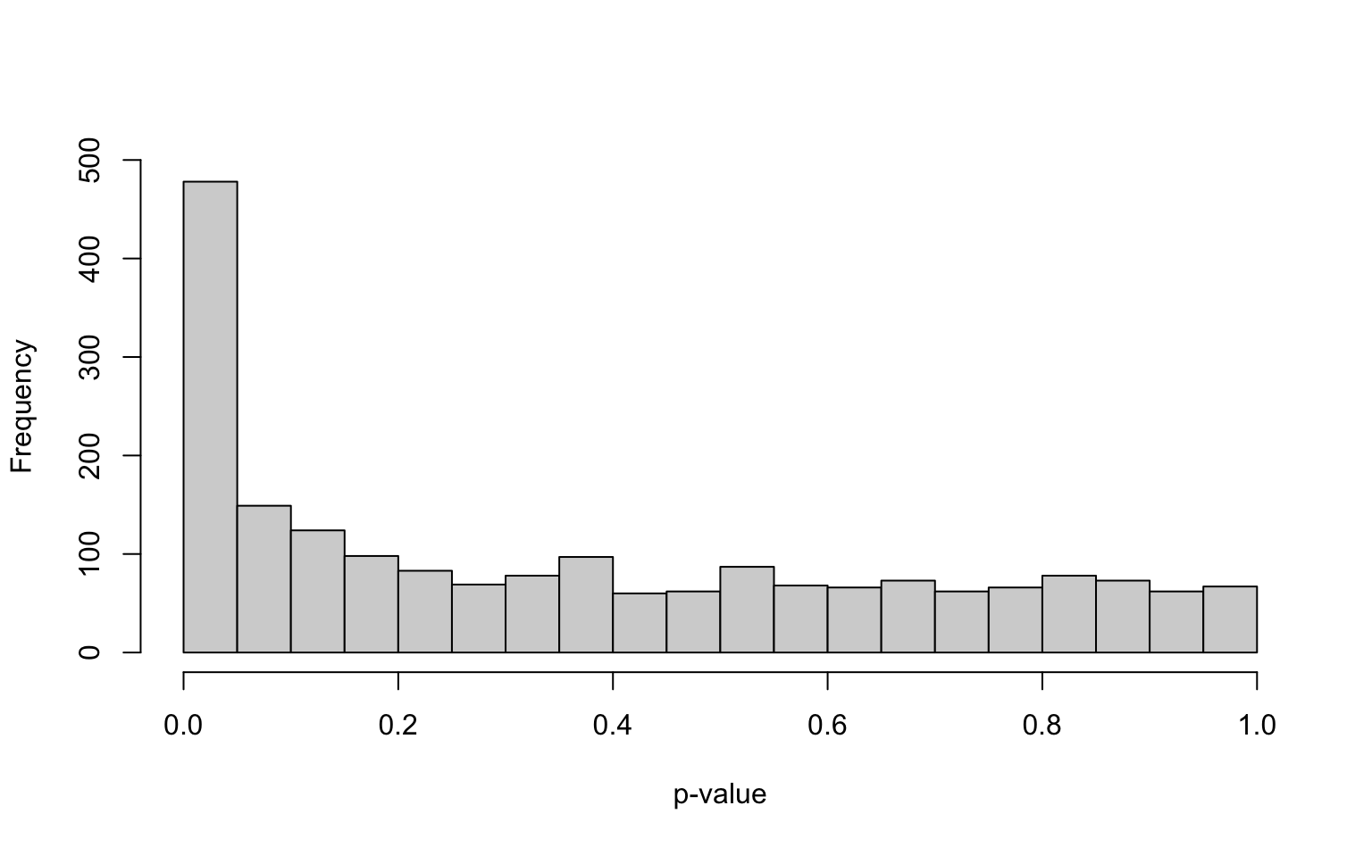
Interpretation: The histogram appears close to a uniform distribution for the larger p-values, but has a lot more small p-values than would be expected under a uniform distribution. Recall that if the null hypothesis (the gene expression is the same for tumor and normal tissue) were to hold for all genes, the p-values would be uniformly distributed on $[0, 1]$.

3. How many discoveries / significant genes do you find when using $\alpha = 0.05$?

Solution

alpha <- 0.05
sum(p_vals <= alpha)
#> [1] 478

4. Control the FWER at 5% using Šidák’s correction. How many genes are significant after the correction?

Solution

m <- nrow(t_test_results)
fwer <- 0.05
adj_alpha <- 1 - (1 - fwer)^(1 / m)

# Number of significant discoveries
sum(p_vals <= adj_alpha)
#> [1] 11

By rearranging the equation $$\alpha = 1 - (1 - \text{FWER})^{1/m} \, ,$$ we can equivalently adjust the p-values via $$1 - (1 - p)^m$$ and compare them to the cut-off 5%:

sidak_p_vals <- 1 - (1 - p_vals)^m

# Number of significant discoveries
sum(sidak_p_vals <= fwer)
#> [1] 11

5. Control the FWER at 5% using the Bonferroni correction. How many genes are significant after the correction?

Solution

By adjusting $\alpha$:

adj_alpha <- fwer / m

# Number of significant discoveries
sum(p_vals <= adj_alpha)
#> [1] 11

Or equivalently, by adjusting the p-values:

bonferroni_p_vals <- p.adjust(p_vals, method = "bonferroni")

# Number of significant discoveries
sum(bonferroni_p_vals <= fwer)
#> [1] 11

6. Control the FDR at 5% using the Benjamini-Hochberg method. How many genes are significant after the correction?

Solution

bh_p_vals <- p.adjust(p_vals, method = "BH")

sum(bh_p_vals < 0.05)
#> [1] 190

7. Plot the adjusted p-values from the Benjamini-Hochberg method against the original p-values. What is the effect of the adjustment?

Bonus: Compute the adjusted p-values based on Šidák’s correction and the Bonferroni correction. Add them to the plot and compare.

Solution

Visualize the adjusted p-values for all three methods in the same figure:

cols <- c("#9d05f4", "#ecd033", "#01d9d9")

plot(
  p_vals[order(p_vals)], bh_p_vals[order(p_vals)],
  pch = 19, cex = 0.6, xlab = "p-value",
  ylab = "Adjusted p-value", col = cols[1]
)
points(
  p_vals[order(p_vals)], bonferroni_p_vals[order(p_vals)],
  pch = 19, cex = 0.6, col = cols[2]
)
points(
  p_vals[order(p_vals)], sidak_p_vals[order(p_vals)],
  pch = 19, cex = 0.6, col = cols[3]
)
abline(a = 0, b = 1)
legend("bottomright",
  c("Benjamini-Hochberg", "Bonferroni", "Sidak"),
  col = cols, pch = 19
)

Interpretation: All three methods adjust the p-values upwards to account for multiple testing. The adjustment is more pronounced for small p-values, while for higher p-values, the curves of the adjusted p-values flatten out. The Benjamini-Hochberg method at a FDR of 5% is less conservative compared to the other two methods. Both Šidák’s correction and the Bonferroni correction at an FWER of 5% adjust the majority of p-values to exactly 1 and only a small proportion of p-values that are originally close to zero remains smaller than 1.

Further reading

• Chapter 6 of the Biomedical Data Science book

Session info

Session info

#> [1] "2025-11-26 17:27:57 CET"
#> ─ Session info ───────────────────────────────────────────────────────────────
#>  setting  value
#>  version  R version 4.5.2 (2025-10-31)
#>  os       macOS Sequoia 15.6
#>  system   aarch64, darwin20
#>  ui       X11
#>  language (EN)
#>  collate  en_US.UTF-8
#>  ctype    en_US.UTF-8
#>  tz       Europe/Brussels
#>  date     2025-11-26
#>  pandoc   3.6.3 @ /Applications/RStudio.app/Contents/Resources/app/quarto/bin/tools/aarch64/ (via rmarkdown)
#>  quarto   1.7.32 @ /Applications/RStudio.app/Contents/Resources/app/quarto/bin/quarto
#> 
#> ─ Packages ───────────────────────────────────────────────────────────────────
#>  package     * version date (UTC) lib source
#>  bookdown      0.45    2025-10-03 [1] CRAN (R 4.5.0)
#>  bslib         0.9.0   2025-01-30 [1] CRAN (R 4.5.0)
#>  cachem        1.1.0   2024-05-16 [1] CRAN (R 4.5.0)
#>  cli           3.6.5   2025-04-23 [1] CRAN (R 4.5.0)
#>  digest        0.6.38  2025-11-12 [1] CRAN (R 4.5.0)
#>  evaluate      1.0.5   2025-08-27 [1] CRAN (R 4.5.0)
#>  fastmap       1.2.0   2024-05-15 [1] CRAN (R 4.5.0)
#>  HDDAData    * 1.0.1   2025-11-06 [1] Github (statOmics/HDDAData@b832c71)
#>  htmltools     0.5.8.1 2024-04-04 [1] CRAN (R 4.5.0)
#>  jquerylib     0.1.4   2021-04-26 [1] CRAN (R 4.5.0)
#>  jsonlite      2.0.0   2025-03-27 [1] CRAN (R 4.5.0)
#>  knitr         1.50    2025-03-16 [1] CRAN (R 4.5.0)
#>  lifecycle     1.0.4   2023-11-07 [1] CRAN (R 4.5.0)
#>  R6            2.6.1   2025-02-15 [1] CRAN (R 4.5.0)
#>  rlang         1.1.6   2025-04-11 [1] CRAN (R 4.5.0)
#>  rmarkdown     2.30    2025-09-28 [1] CRAN (R 4.5.0)
#>  rstudioapi    0.17.1  2024-10-22 [1] CRAN (R 4.5.0)
#>  sass          0.4.10  2025-04-11 [1] CRAN (R 4.5.0)
#>  sessioninfo   1.2.3   2025-02-05 [1] CRAN (R 4.5.0)
#>  xfun          0.54    2025-10-30 [1] CRAN (R 4.5.0)
#>  yaml          2.3.10  2024-07-26 [1] CRAN (R 4.5.0)
#> 
#>  [1] /Library/Frameworks/R.framework/Versions/4.5-arm64/Resources/library
#>  * ── Packages attached to the search path.
#> 
#> ──────────────────────────────────────────────────────────────────────────────

References

Alon, Uri, Naama Barkai, Daniel A Notterman, Kurt Gish, Suzanne Ybarra, Daniel Mack, and Arnold J Levine. 1999. “Broad Patterns of Gene Expression Revealed by Clustering Analysis of Tumor and Normal Colon Tissues Probed by Oligonucleotide Arrays.” Proceedings of the National Academy of Sciences 96 (12): 6745–50.

---

This work is licensed under the CC BY-NC-SA 4.0 licence.