Lab 5: Clustering

High Dimensional Data Analysis practicals

Change log

---

## Install necessary packages with:

# install.packages(c("mclust", "gclus", "tidyverse", "gridExtra"))

# if (!requireNamespace("remotes", quietly = TRUE)) {
#     install.packages("remotes")
# }
# remotes::install_github("vqv/ggbiplot")

library(mclust)
library(gclus)  # contains the 'wine' data
library(ggbiplot)
library(tidyverse)
library(gridExtra)

theme_set(theme_minimal())

1 The wine data

In this lab session, we will explore the wine data, following the example analysis from Scrucca et al. (2016).

This dataset provides 13 measurements obtained from a chemical analysis of 178 wines grown in the same region in Italy but derived from three different cultivars (Barolo, Grignolino, Barbera). The original cultivar labels are provided in the dataset.

We will apply different clustering algorithms and validate them by comparing how well the clusters capture the original classes.

data("wine", package = "gclus")
class <- factor(wine$Class, levels = 1:3, labels = c("Barolo", "Grignolino", "Barbera"))
table(class)
#> class
#>     Barolo Grignolino    Barbera 
#>         59         71         48

X <- as.matrix(wine[, -1])
summary(X)
#>     Alcohol          Malic            Ash          Alcalinity   
#>  Min.   :11.03   Min.   :0.740   Min.   :1.360   Min.   :10.60  
#>  1st Qu.:12.36   1st Qu.:1.603   1st Qu.:2.210   1st Qu.:17.20  
#>  Median :13.05   Median :1.865   Median :2.360   Median :19.50  
#>  Mean   :13.00   Mean   :2.336   Mean   :2.367   Mean   :19.49  
#>  3rd Qu.:13.68   3rd Qu.:3.083   3rd Qu.:2.558   3rd Qu.:21.50  
#>  Max.   :14.83   Max.   :5.800   Max.   :3.230   Max.   :30.00  
#>    Magnesium         Phenols        Flavanoids     Nonflavanoid   
#>  Min.   : 70.00   Min.   :0.980   Min.   :0.340   Min.   :0.1300  
#>  1st Qu.: 88.00   1st Qu.:1.742   1st Qu.:1.205   1st Qu.:0.2700  
#>  Median : 98.00   Median :2.355   Median :2.135   Median :0.3400  
#>  Mean   : 99.74   Mean   :2.295   Mean   :2.029   Mean   :0.3619  
#>  3rd Qu.:107.00   3rd Qu.:2.800   3rd Qu.:2.875   3rd Qu.:0.4375  
#>  Max.   :162.00   Max.   :3.880   Max.   :5.080   Max.   :0.6600  
#>  Proanthocyanins   Intensity           Hue             OD280      
#>  Min.   :0.410   Min.   : 1.280   Min.   :0.4800   Min.   :1.270  
#>  1st Qu.:1.250   1st Qu.: 3.220   1st Qu.:0.7825   1st Qu.:1.938  
#>  Median :1.555   Median : 4.690   Median :0.9650   Median :2.780  
#>  Mean   :1.591   Mean   : 5.058   Mean   :0.9575   Mean   :2.612  
#>  3rd Qu.:1.950   3rd Qu.: 6.200   3rd Qu.:1.1200   3rd Qu.:3.170  
#>  Max.   :3.580   Max.   :13.000   Max.   :1.7100   Max.   :4.000  
#>     Proline      
#>  Min.   : 278.0  
#>  1st Qu.: 500.5  
#>  Median : 673.5  
#>  Mean   : 746.9  
#>  3rd Qu.: 985.0  
#>  Max.   :1680.0

We will use a PCA to visualize the data, along with the class labels, in a low-dimensional space. This will allow us to interpret the results of the clustering algorithms more easily.

Tasks

1. Perform a PCA of the scaled wine data.

Solution

wine_pca <- prcomp(X, scale. = TRUE)

2. Create a biplot of the first two PCs. Color each observation by its class label. Interpret the PCs. How distinguishable are the classes with respect to the PCs?

Solution

Using ggbiplot:

cols <- c("Barolo" = "#28a028", "Grignolino" = "#da6852", "Barbera" = "#0078cd")

ggbiplot(wine_pca, groups = class) +
  scale_color_manual(values = cols) +
  labs(color = "True labels") +
  theme(aspect.ratio = 0.8, legend.position = "top")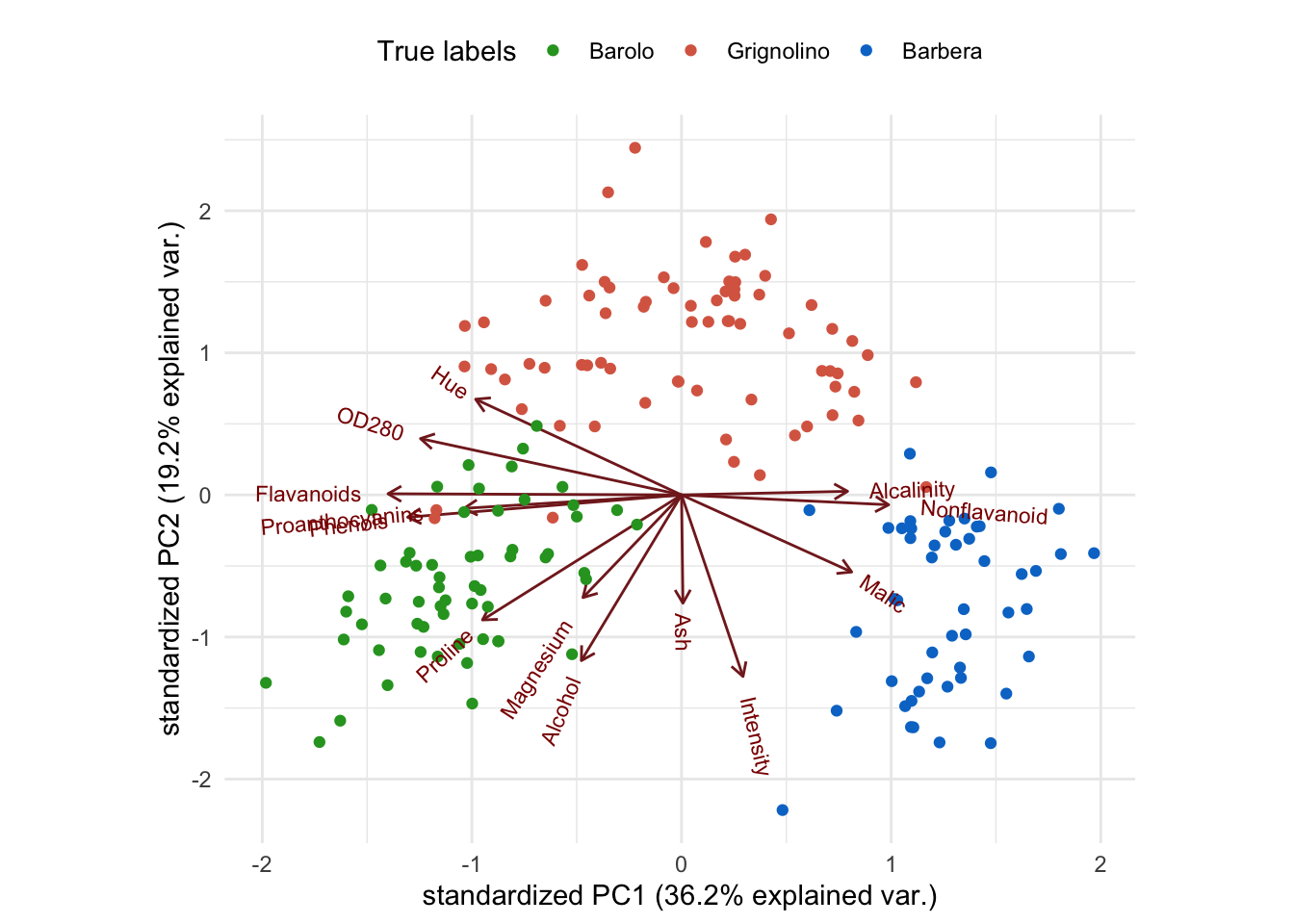

Alternatively, using base R plotting:

Zk <- wine_pca$x[, 1:2]
Vk <- wine_pca$rotation[, 1:2]

plot(Zk, pch = 20,
  col = cols[class],
  xlab = "PC1", ylab = "PC2"
)
legend("topleft", levels(class),
  col = cols,
  pch = 19
)
alpha <- 5 # rescaling
for (i in 1:13) {
  arrows(0, 0, alpha * Vk[i, 1], alpha * Vk[i, 2], length = 0.2, col = "#8f4040")
  text(alpha * Vk[i, 1], alpha * Vk[i, 2], rownames(Vk)[i], col = "#8f4040")
}

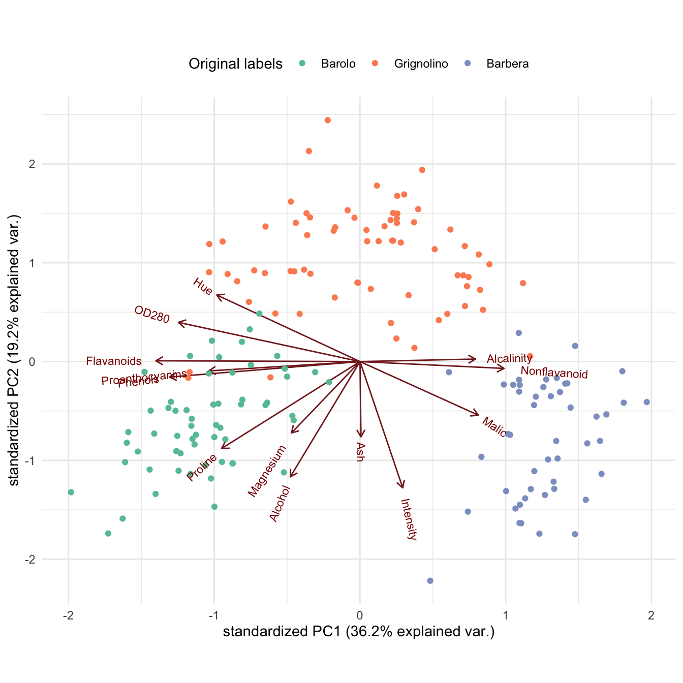
Interpretation: Low values on PC1 correspond to heavier, aged, more structured wines, while high values indicate fresher, less heavy, younger wines. High values on PC2 correspond to lighter-colored wines with lower alcohol content. Importantly, the three classes are quite clearly visually separated with little overlap between them. We can thus rely on the biplot to visually investigate how well a clustering algorithm recovers the true classes.

2 Hierarchical clustering

Tasks

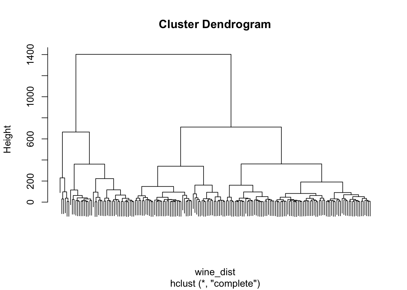
1. Perform hierarchical clustering of the wine data, using a Euclidean distance matrix and the complete-linkage algorithm (see ?hclust).

Solution

# Calculate distance matrix and perform hierarchical clustering
wine_dist <- dist(X, method = "euclidean")
hc <- hclust(wine_dist, method = "complete")

2. Plot the clustering dendrogram.

Solution

plot(hc, labels = FALSE)

3. Use cutree to select three clusters from the hierarchical clustering. Recreate the PCA biplot from Section 1, but color each observation according to its cluster. Compare the resulting biplot to the earlier one from Section 1.

Solution

# Select three clusters
hc_clusters <- cutree(hc, k = 3)
# Tabulate clusters against true classes
table(class, hc_clusters)
#>             hc_clusters
#> class         1  2  3
#>   Barolo     43 16  0
#>   Grignolino  0 15 56
#>   Barbera     0 21 27

Biplot with ggbiplot:

plot1 <- ggbiplot(wine_pca, groups = class) +
  scale_color_manual(values = cols) +
  labs(color = "True labels") +
  theme(aspect.ratio = 0.8, legend.position = "top")

plot2 <- ggbiplot(wine_pca, groups = factor(hc_clusters)) +
  scale_color_manual(values = c("#9d05f4", "#01d9d9", "#f4dc00")) +
  labs(color = "HC clusters") +
  theme(aspect.ratio = 0.8, legend.position = "top")

grid.arrange(plot1, nullGrob(), plot2, ncol = 3, widths = c(1, 0.1, 1))

Alternatively, using base R plotting:

par(mfrow = c(1, 2))

# True class labels
plot(Zk, pch = 20,
  col = cols[class],
  xlab = "PC1", ylab = "PC2"
)
legend("topleft", levels(class),
  col = cols,
  pch = 19
)
alpha <- 5 # rescaling
for (i in 1:13) {
  arrows(0, 0, alpha * Vk[i, 1], alpha * Vk[i, 2], length = 0.2, col = "#8f4040")
  text(alpha * Vk[i, 1], alpha * Vk[i, 2], rownames(Vk)[i], col = "#8f4040")
}

cluster_cols <- c("1" = "#9d05f4", "2" = "#01d9d9", "3" = "#f4dc00")
# Clusters
plot(Zk, pch = 20,
  col = cluster_cols[factor(hc_clusters)],
  xlab = "PC1", ylab = "PC2"
)
legend("topleft", levels(factor(hc_clusters)),
  col = cluster_cols,
  pch = 19
)
alpha <- 5 # rescaling
for (i in 1:13) {
  arrows(0, 0, alpha * Vk[i, 1], alpha * Vk[i, 2], length = 0.2, col = "#8f4040")
  text(alpha * Vk[i, 1], alpha * Vk[i, 2], rownames(Vk)[i], col = "#8f4040")
}

Interpretation: The first cluster corresponds to most of the Barolo class, but the second cluster overlaps with all three classes, and the third cluster captures wines from both the Grignolino and the Barbera class. Overall, the three clusters do not recover the true class labels.

Bonus: can you improve the results by using different distance metrics or linkages?

3 Model-based clustering

Tasks

1. Use mclust::Mclust() to perform model-based clustering on the wine data.

Solution

mc <- Mclust(X)
summary(mc)
#> ---------------------------------------------------- 
#> Gaussian finite mixture model fitted by EM algorithm 
#> ---------------------------------------------------- 
#> 
#> Mclust VVE (ellipsoidal, equal orientation) model with 3 components: 
#> 
#>  log-likelihood   n  df       BIC       ICL
#>       -3015.335 178 158 -6849.391 -6850.734
#> 
#> Clustering table:
#>  1  2  3 
#> 59 69 50
summary(mc$BIC)
#> Best BIC values:
#>              VVE,3       EVE,4       VVE,4
#> BIC      -6849.391 -6873.61648 -6885.47222
#> BIC diff     0.000   -24.22499   -36.08073

2. Visualize the clustering via pairwise plots. Plot the BIC (Bayesian information criterion) values and interpret the results.

Hint: Check ?plot.Mclust.

Solution

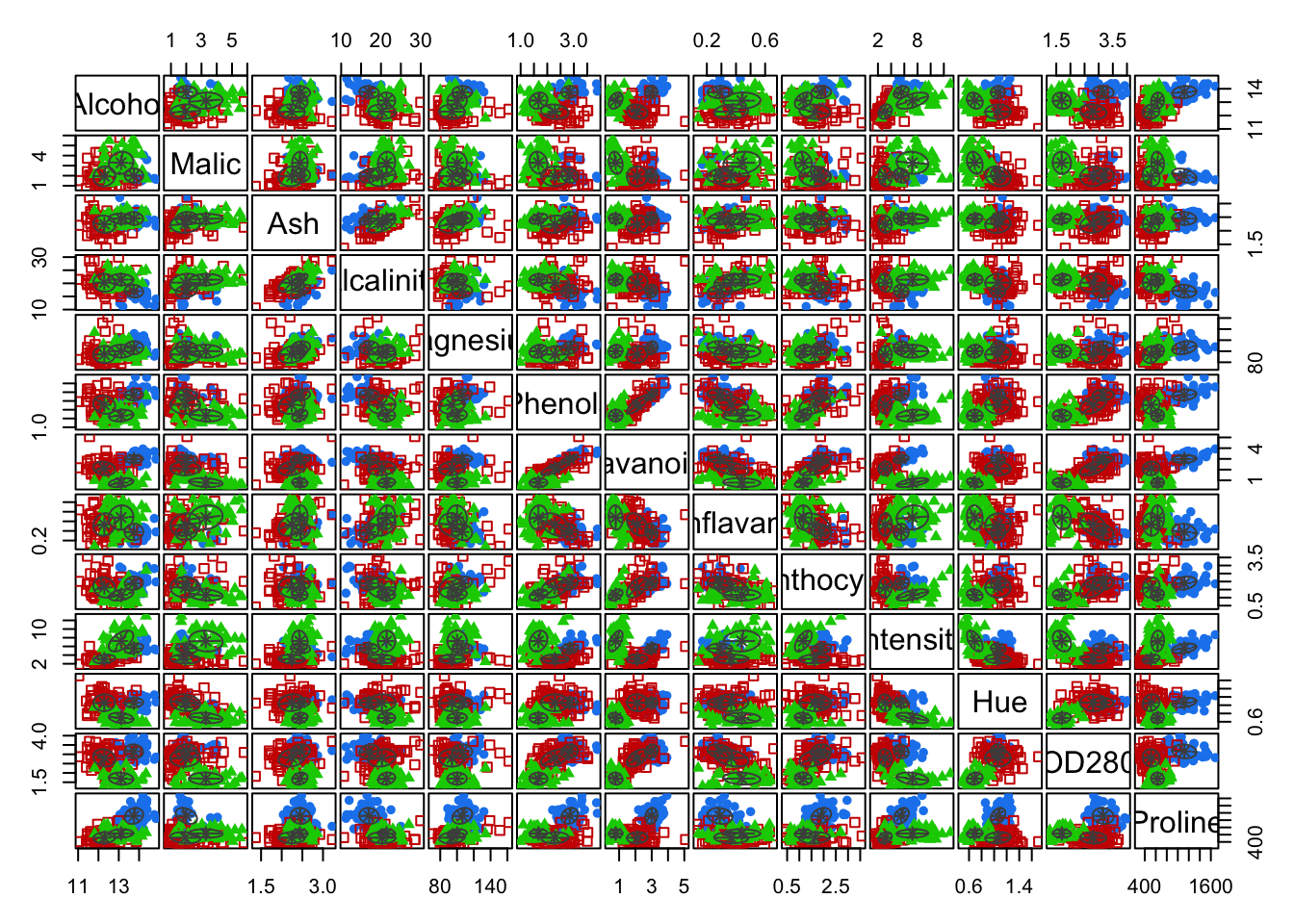
# Pairwise clustering plots
plot(mc, what = "classification")

# BIC plot; exclude two models with very low BIC
plot(mc, what = "BIC", ylim = range(mc$BIC[, -(1:2)], na.rm = TRUE),
  legendArgs = list(x = "bottomleft")
)

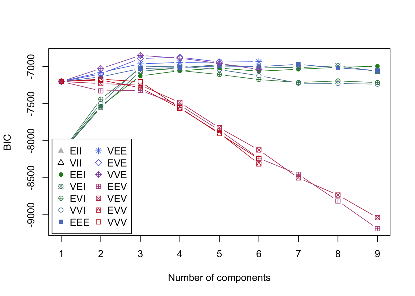
Interpretation: A three-component mixture with covariances having different shapes and volumes but the same orientation (VVE) results in the highest BIC.

3. Recreate the PCA biplot from Section 1, but color each observation according to its cluster. Compare the resulting biplot to the earlier ones.

Solution

# Tabulate clusters against true classes
table(class, mc$classification)
#>             
#> class         1  2  3
#>   Barolo     59  0  0
#>   Grignolino  0 69  2
#>   Barbera     0  0 48

Biplot with ggbiplot:

plot1 <- ggbiplot(wine_pca, groups = class) +
  scale_color_manual(values = cols) +
  labs(color = "True labels") +
  theme(aspect.ratio = 0.8, legend.position = "top")

plot2 <- ggbiplot(wine_pca, groups = factor(mc$classification)) +
  scale_color_manual(values = c("#9d05f4", "#01d9d9", "#f4dc00")) +
  labs(color = "Mclust clusters") +
  theme(aspect.ratio = 0.8, legend.position = "top")

grid.arrange(plot1, nullGrob(), plot2, ncol = 3, widths = c(1, 0.1, 1))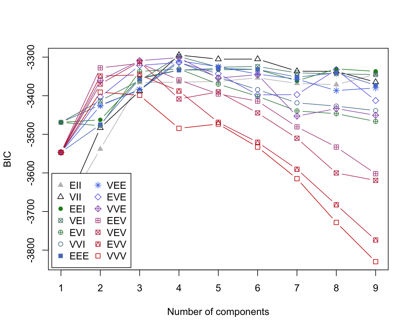

Alternatively, using base R plotting:

par(mfrow = c(1, 2))

# True class labels
plot(Zk, pch = 20,
  col = cols[class],
  xlab = "PC1", ylab = "PC2"
)
legend("topleft", levels(class),
  col = cols,
  pch = 19
)
alpha <- 5 # rescaling
for (i in 1:13) {
  arrows(0, 0, alpha * Vk[i, 1], alpha * Vk[i, 2], length = 0.2, col = "#8f4040")
  text(alpha * Vk[i, 1], alpha * Vk[i, 2], rownames(Vk)[i], col = "#8f4040")
}

cluster_cols <- c("1" = "#9d05f4", "2" = "#01d9d9", "3" = "#f4dc00")
# Clusters
plot(Zk, pch = 20,
  col = cluster_cols[factor(mc$classification)],
  xlab = "PC1", ylab = "PC2"
)
legend("topleft", levels(factor(mc$classification)),
  col = cluster_cols,
  pch = 19
)
alpha <- 5 # rescaling
for (i in 1:13) {
  arrows(0, 0, alpha * Vk[i, 1], alpha * Vk[i, 2], length = 0.2, col = "#8f4040")
  text(alpha * Vk[i, 1], alpha * Vk[i, 2], rownames(Vk)[i], col = "#8f4040")
}

Interpretation: The first cluster corresponds to the Barolo class, the second cluster to the Grignolino class and the third cluster to Barbera. Overall, the three clusters recover the true class labels very well, with only two Grignolino wines falsely assigned to the third cluster (Barbera).

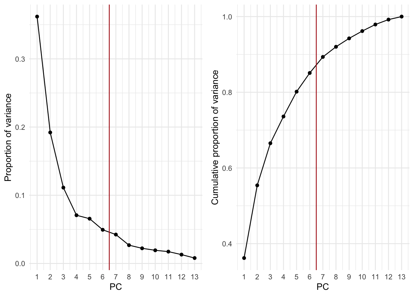
4. Select an appropriate number of PCs from the PCA. Repeat the model-based clustering on the PCs. How do the results compare to those on the full data?

Solution

# Proportion of variance explained by each PC
wine_prop_var <- data.frame(
  PC = 1:ncol(wine_pca$x),
  var = wine_pca$sdev^2 / sum(wine_pca$sdev^2)
)

ggplot(wine_prop_var, aes(PC, var)) +
  geom_point() +
  geom_line() +
  geom_vline(xintercept = 7.5, col = "firebrick") +
  scale_x_continuous(breaks = 1:ncol(wine_pca$x)) +
  labs(y = "Proportion of variance")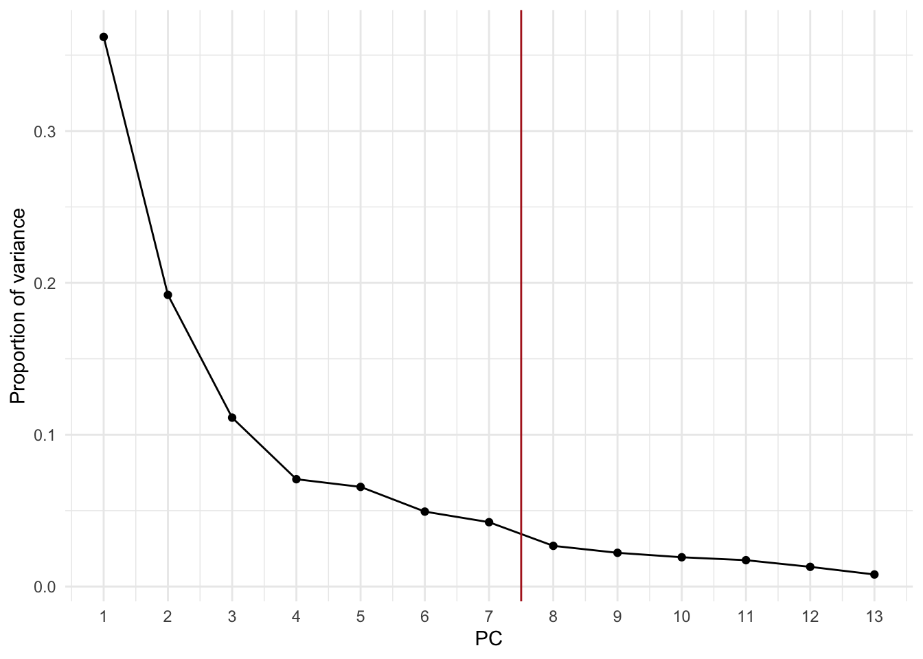

The first 7 PCs explain about 92% of the variance in the wine data.

# Select the first k PCs
k <- 7
pca_X <- wine_pca$x[, 1:k]

# Refit the model-based clustering
mc2 <- Mclust(pca_X)
summary(mc2)
#> ---------------------------------------------------- 
#> Gaussian finite mixture model fitted by EM algorithm 
#> ---------------------------------------------------- 
#> 
#> Mclust VEI (diagonal, equal shape) model with 5 components: 
#> 
#>  log-likelihood   n df       BIC       ICL
#>       -1719.764 178 50 -3698.617 -3725.317
#> 
#> Clustering table:
#>  1  2  3  4  5 
#> 53 25 19 34 47
summary(mc2$BIC)
#> Best BIC values:
#>              VEI,5        VEI,4        VEI,6
#> BIC      -3698.617 -3700.939851 -3704.927637
#> BIC diff     0.000    -2.322571    -6.310357

A five-component mixture with diagonal covariances having equal shape, but varying volume (VEI), results in the highest BIC.

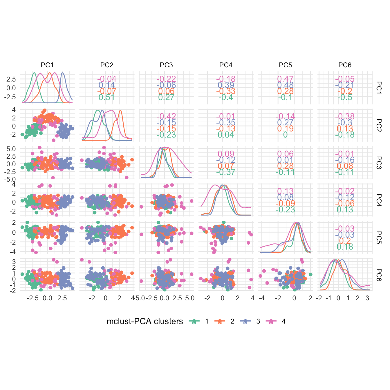
# Tabulate clusters against true classes
table(class, mc2$classification)
#>             
#> class         1  2  3  4  5
#>   Barolo     53  6  0  0  0
#>   Grignolino  0 16 18 34  3
#>   Barbera     0  3  1  0 44

Biplot with ggbiplot:

plot1 <- ggbiplot(wine_pca, groups = class) +
  scale_color_manual(values = cols) +
  labs(color = "True labels") +
  theme(aspect.ratio = 0.8, legend.position = "top")

plot2 <- ggbiplot(wine_pca, groups = factor(mc2$classification)) +
  scale_color_manual(values = c("#9d05f4", "#01d9d9", "#01d9d9", "#01d9d9", "#f4dc00")) +
  labs(color = "Mclust clusters") +
  theme(aspect.ratio = 0.8, legend.position = "top")

grid.arrange(plot1, nullGrob(), plot2, ncol = 3, widths = c(1, 0.1, 1))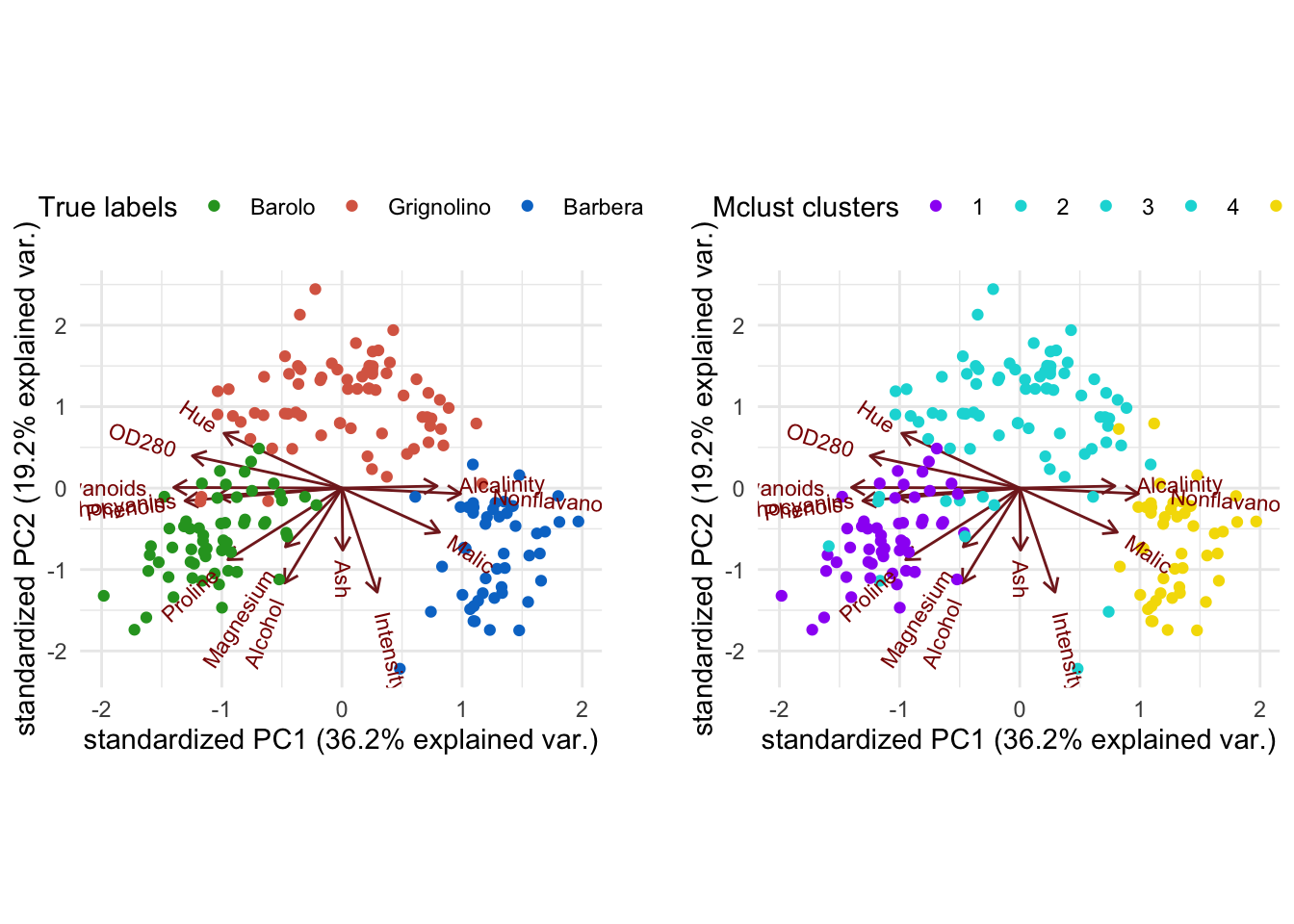

Alternatively, using base R plotting:

par(mfrow = c(1, 2))

# True class labels
plot(Zk, pch = 20,
  col = cols[class],
  xlab = "PC1", ylab = "PC2"
)
legend("topleft", levels(class),
  col = cols,
  pch = 19
)
alpha <- 5 # rescaling
for (i in 1:13) {
  arrows(0, 0, alpha * Vk[i, 1], alpha * Vk[i, 2], length = 0.2, col = "#8f4040")
  text(alpha * Vk[i, 1], alpha * Vk[i, 2], rownames(Vk)[i], col = "#8f4040")
}

cluster_cols <- c("1" = "#9d05f4", "2" = "#01d9d9", "3" = "#01d9d9", "4" = "#01d9d9", "5" = "#f4dc00")
# Clusters
plot(Zk, pch = 20,
  col = cluster_cols[factor(mc2$classification)],
  xlab = "PC1", ylab = "PC2"
)
legend("topleft", levels(factor(mc2$classification)),
  col = cluster_cols,
  pch = 19
)
alpha <- 5 # rescaling
for (i in 1:13) {
  arrows(0, 0, alpha * Vk[i, 1], alpha * Vk[i, 2], length = 0.2, col = "#8f4040")
  text(alpha * Vk[i, 1], alpha * Vk[i, 2], rownames(Vk)[i], col = "#8f4040")
}

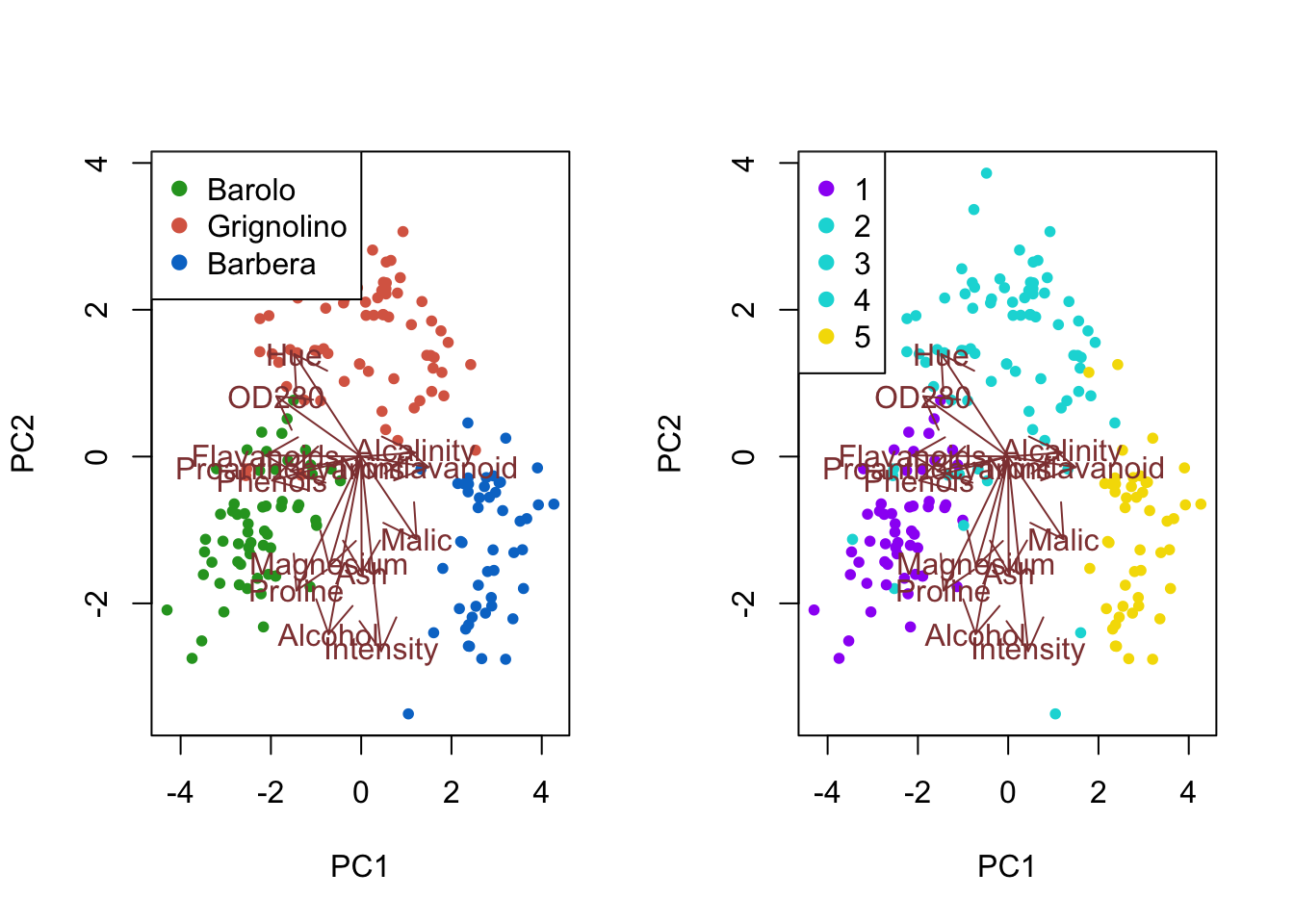
Interpretation: The first cluster corresponds to most of the Barolo class. The fifth color mainly corresponds to the Barbera class, while containing a few Grignolino wines. Combining the second, third and fourth cluster recovers most of the Grignolino class, with some overlap with the remaining classes. Overall, after combining the three smaller clusters, the clustering recovers the true class labels fairly well, though not quite as closely as the clustering on the original data.

Additional resources

• Section 14.3 of Hastie, Tibshirani, and Friedman (2009)

Session info

Session info

#> [1] "2025-11-09 16:06:01 CET"
#> ─ Session info ───────────────────────────────────────────────────────────────
#>  setting  value
#>  version  R version 4.5.2 (2025-10-31)
#>  os       macOS Sequoia 15.6
#>  system   aarch64, darwin20
#>  ui       X11
#>  language (EN)
#>  collate  en_US.UTF-8
#>  ctype    en_US.UTF-8
#>  tz       Europe/Brussels
#>  date     2025-11-09
#>  pandoc   3.6.3 @ /Applications/RStudio.app/Contents/Resources/app/quarto/bin/tools/aarch64/ (via rmarkdown)
#>  quarto   1.7.32 @ /Applications/RStudio.app/Contents/Resources/app/quarto/bin/quarto
#> 
#> ─ Packages ───────────────────────────────────────────────────────────────────
#>  package      * version date (UTC) lib source
#>  bookdown       0.45    2025-10-03 [1] CRAN (R 4.5.0)
#>  bslib          0.9.0   2025-01-30 [1] CRAN (R 4.5.0)
#>  cachem         1.1.0   2024-05-16 [1] CRAN (R 4.5.0)
#>  cli            3.6.5   2025-04-23 [1] CRAN (R 4.5.0)
#>  cluster      * 2.1.8.1 2025-03-12 [1] CRAN (R 4.5.2)
#>  digest         0.6.37  2024-08-19 [1] CRAN (R 4.5.0)
#>  dplyr        * 1.1.4   2023-11-17 [1] CRAN (R 4.5.0)
#>  evaluate       1.0.5   2025-08-27 [1] CRAN (R 4.5.0)
#>  farver         2.1.2   2024-05-13 [1] CRAN (R 4.5.0)
#>  fastmap        1.2.0   2024-05-15 [1] CRAN (R 4.5.0)
#>  forcats      * 1.0.1   2025-09-25 [1] CRAN (R 4.5.0)
#>  gclus        * 1.3.3   2025-03-28 [1] CRAN (R 4.5.0)
#>  generics       0.1.4   2025-05-09 [1] CRAN (R 4.5.0)
#>  ggbiplot     * 0.55    2025-11-05 [1] Github (vqv/ggbiplot@f7ea76d)
#>  ggplot2      * 4.0.0   2025-09-11 [1] CRAN (R 4.5.0)
#>  glue           1.8.0   2024-09-30 [1] CRAN (R 4.5.0)
#>  gridExtra    * 2.3     2017-09-09 [1] CRAN (R 4.5.0)
#>  gtable         0.3.6   2024-10-25 [1] CRAN (R 4.5.0)
#>  hms            1.1.4   2025-10-17 [1] CRAN (R 4.5.0)
#>  htmltools      0.5.8.1 2024-04-04 [1] CRAN (R 4.5.0)
#>  jquerylib      0.1.4   2021-04-26 [1] CRAN (R 4.5.0)
#>  jsonlite       2.0.0   2025-03-27 [1] CRAN (R 4.5.0)
#>  knitr          1.50    2025-03-16 [1] CRAN (R 4.5.0)
#>  labeling       0.4.3   2023-08-29 [1] CRAN (R 4.5.0)
#>  lifecycle      1.0.4   2023-11-07 [1] CRAN (R 4.5.0)
#>  lubridate    * 1.9.4   2024-12-08 [1] CRAN (R 4.5.0)
#>  magrittr       2.0.4   2025-09-12 [1] CRAN (R 4.5.0)
#>  mclust       * 6.1.2   2025-10-31 [1] CRAN (R 4.5.0)
#>  pillar         1.11.1  2025-09-17 [1] CRAN (R 4.5.0)
#>  pkgconfig      2.0.3   2019-09-22 [1] CRAN (R 4.5.0)
#>  plyr         * 1.8.9   2023-10-02 [1] CRAN (R 4.5.0)
#>  purrr        * 1.2.0   2025-11-04 [1] CRAN (R 4.5.0)
#>  R6             2.6.1   2025-02-15 [1] CRAN (R 4.5.0)
#>  RColorBrewer   1.1-3   2022-04-03 [1] CRAN (R 4.5.0)
#>  Rcpp           1.1.0   2025-07-02 [1] CRAN (R 4.5.0)
#>  readr        * 2.1.5   2024-01-10 [1] CRAN (R 4.5.0)
#>  rlang          1.1.6   2025-04-11 [1] CRAN (R 4.5.0)
#>  rmarkdown      2.30    2025-09-28 [1] CRAN (R 4.5.0)
#>  rstudioapi     0.17.1  2024-10-22 [1] CRAN (R 4.5.0)
#>  S7             0.2.0   2024-11-07 [1] CRAN (R 4.5.0)
#>  sass           0.4.10  2025-04-11 [1] CRAN (R 4.5.0)
#>  scales       * 1.4.0   2025-04-24 [1] CRAN (R 4.5.0)
#>  sessioninfo    1.2.3   2025-02-05 [1] CRAN (R 4.5.0)
#>  stringi        1.8.7   2025-03-27 [1] CRAN (R 4.5.0)
#>  stringr      * 1.6.0   2025-11-04 [1] CRAN (R 4.5.0)
#>  tibble       * 3.3.0   2025-06-08 [1] CRAN (R 4.5.0)
#>  tidyr        * 1.3.1   2024-01-24 [1] CRAN (R 4.5.0)
#>  tidyselect     1.2.1   2024-03-11 [1] CRAN (R 4.5.0)
#>  tidyverse    * 2.0.0   2023-02-22 [1] CRAN (R 4.5.0)
#>  timechange     0.3.0   2024-01-18 [1] CRAN (R 4.5.0)
#>  tzdb           0.5.0   2025-03-15 [1] CRAN (R 4.5.0)
#>  vctrs          0.6.5   2023-12-01 [1] CRAN (R 4.5.0)
#>  withr          3.0.2   2024-10-28 [1] CRAN (R 4.5.0)
#>  xfun           0.54    2025-10-30 [1] CRAN (R 4.5.0)
#>  yaml           2.3.10  2024-07-26 [1] CRAN (R 4.5.0)
#> 
#>  [1] /Library/Frameworks/R.framework/Versions/4.5-arm64/Resources/library
#>  * ── Packages attached to the search path.
#> 
#> ──────────────────────────────────────────────────────────────────────────────

References

Hastie, Trevor, Robert Tibshirani, and Jerome Friedman. 2009. The Elements of Statistical Learning. 2nd ed. Springer.

---

This work is licensed under the CC BY-NC-SA 4.0 licence.