9. Non-parametric statistics - Kruskal Wallis

1 Comparison of \(g\) groups

• Extend \(F\)-test from a one-way ANOVA to non-parametric alternatives.

2 DMH example

Assess genotoxicity of 1,2-dimethylhydrazine dihydrochloride (DMH) (EU directive)

• 24 rats
• four groups with daily DMH dose
  • control
  • low
  • medium
  • high
• Genotoxicity in liver using comet assay on 150 liver cells per rat.
• Are there differences in DNA damage due to DMH dose?

2.1 Comet Assay:

• Visualise DNA strand breaks
• Length comet tail is a proxy for strand breaks.

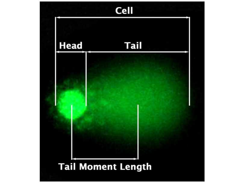
Comet assay

dna <- read_delim("https://raw.githubusercontent.com/GTPB/PSLS20/master/data/dna.txt", delim = " ")
dna$dose <- as.factor(dna$dose)
dna

dna %>%
  ggplot(aes(x = dose, y = length, fill = dose)) +
  geom_boxplot() +
  geom_point(position = "jitter")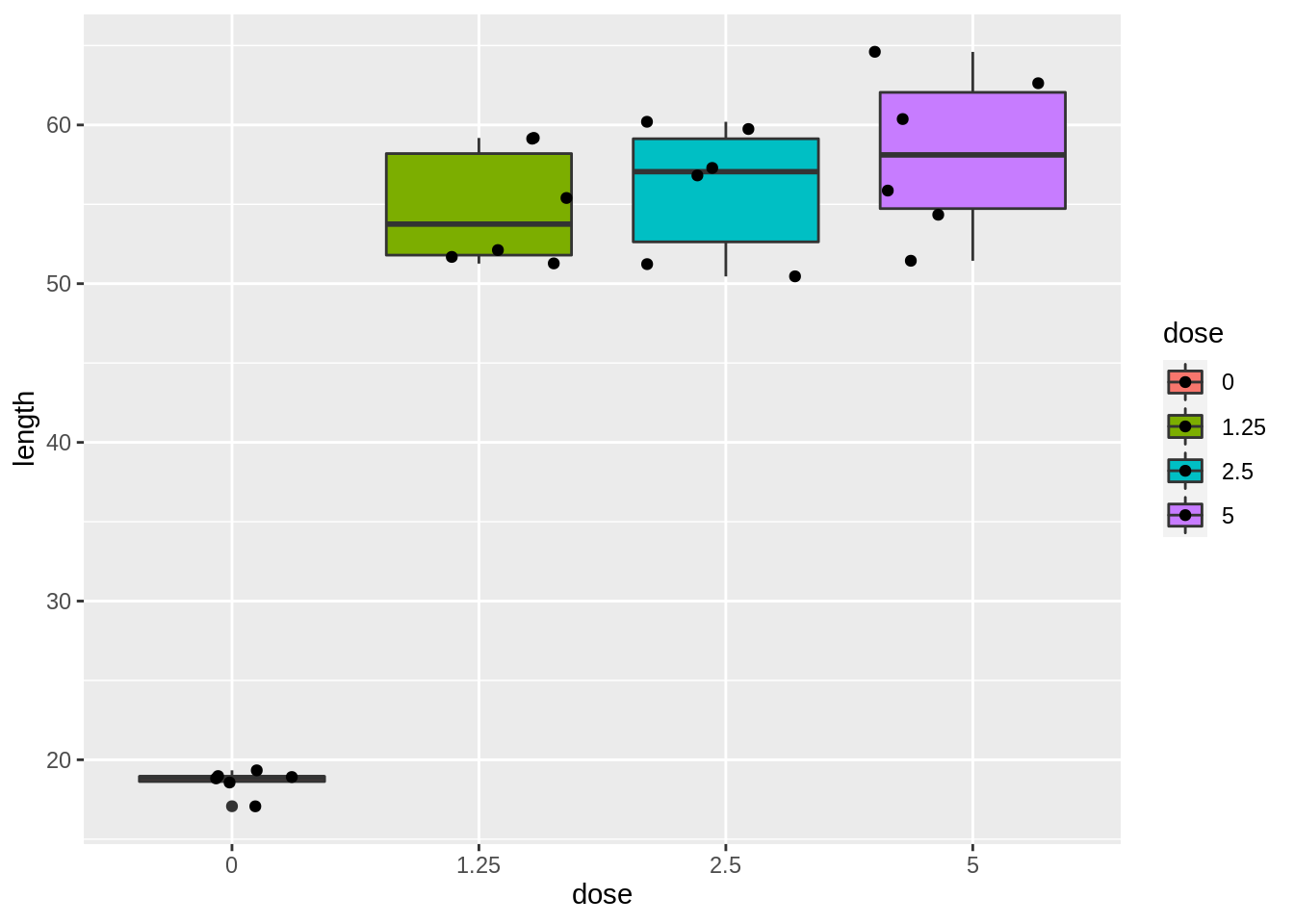

dna %>%
  ggplot(aes(sample = length)) +
  geom_qq() +
  geom_qq_line() +
  facet_wrap(~dose)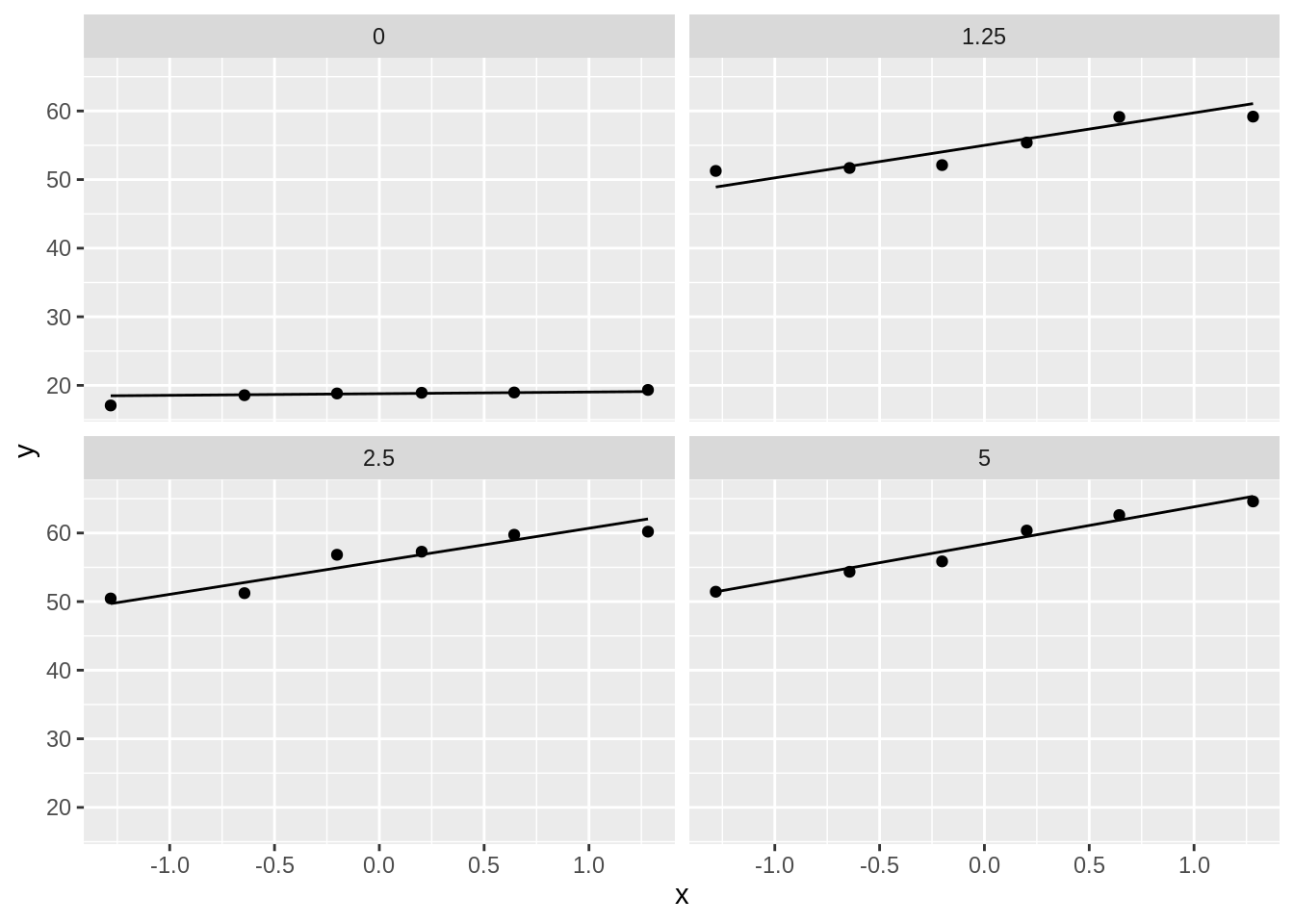

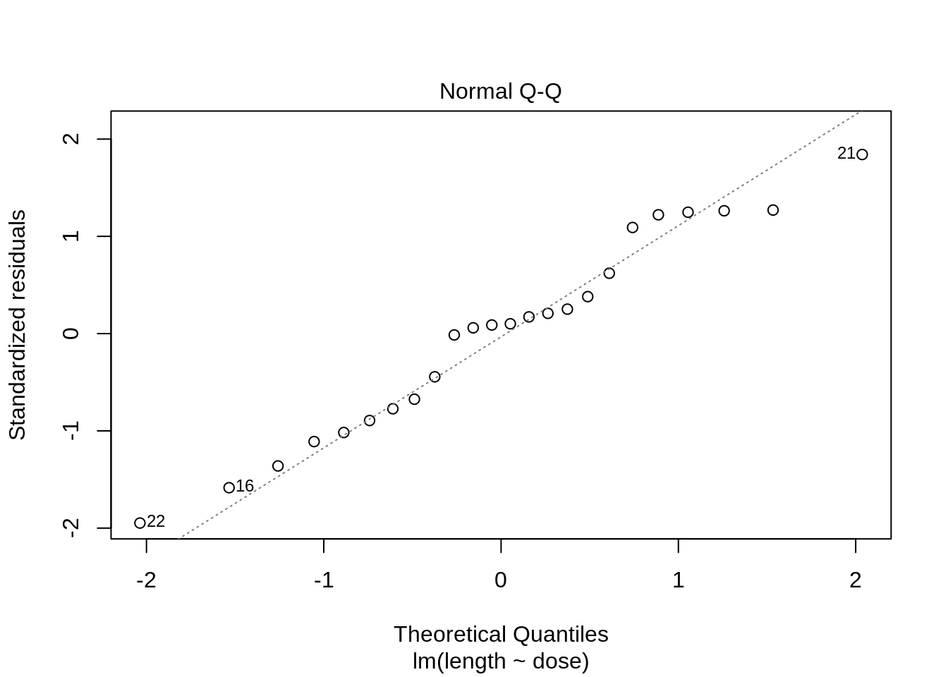
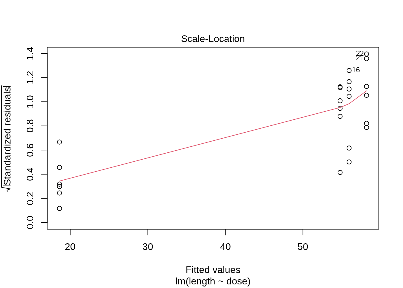
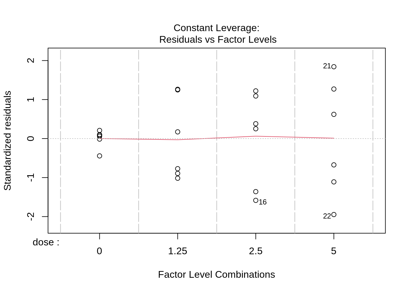
• Strong indication that data in control group has a lower variance.
• 6 observations per group are too few to check the assumptions

plot(lm(length ~ dose, data = dna))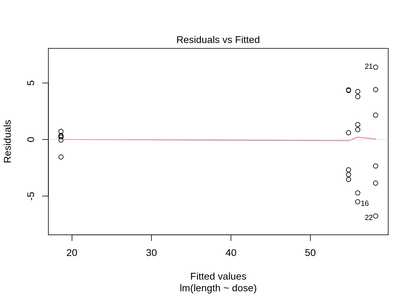

3 Kruskal-Wallis Rank Test

• The Kruskal-Wallis Rank Test (KW-test) is a non-parameteric alternative for ANOVA F-test.

• Classical \(F\)-teststatistic can be written as \[ F = \frac{\text{SST}/(g-1)}{\text{SSE}/(n-g)} = \frac{\text{SST}/(g-1)}{(\text{SSTot}-\text{SST})/(n-g)} , \]

• with \(g\) the number of groups.

• SSTot depends only on outcomes \(\mathbf{y}\) and will not vary in permutation test.

• SST can be used as statistic \[\text{SST}=\sum_{j=1}^t n_j(\bar{Y}_j-\bar{Y})^2\]

• The KW test statistic is based on SST on rank-transformed outcomes¹, \[ \text{SST} = \sum_{j=1}^g n_j \left(\bar{R}_j - \bar{R}\right)^2 = \sum_{j=1}^t n_j \left(\bar{R}_j - \frac{n+1}{2}\right)^2 , \]

• with \(\bar{R}_j\) the mean of the ranks in group \(j\), and \(\bar{R}\) the mean of all ranks, \[ \bar{R} = \frac{1}{n}(1+2+\cdots + n) = \frac{1}{n}\frac{1}{2}n(n+1) = \frac{n+1}{2}. \]

• The KW teststatistic is given by \[ KW = \frac{12}{n(n+1)} \sum_{j=1}^g n_j \left(\bar{R}_j - \frac{n+1}{2}\right)^2. \]

• The factor \(\frac{12}{n(n+1)}\) is used so that \(KW\) has a simple asymptotic null distribution. In particular under \(H_0\), given thart \(\min(n_1,\ldots, n_g)\rightarrow \infty\), \[ KW \rightarrow \chi^2_{t-1}. \]

• The exact KW-test can be executed by calculating the permutation null distribution (that only depends on \(n_1, \ldots, n_g\)) to test \[H_0: f_1=\ldots=f_g \text{ vs } H_1: \text{ at least two means are different}.\]

• In order to allow \(H_1\) to be formulated in terms of means, the assumption of locations shift should be valid.

• For DMH example this is not the case.

• If location-shift is invalid, we have to formulate \(H_1\) in terms of probabilistic indices: \[H_0: f_1=\ldots=f_g \text{ vs } H_1: \exists\ j,k \in \{1,\ldots,g\} : \text{P}\left[Y_j\geq Y_k\right]\neq 0.5\]

3.1 DNA Damage Example

kruskal.test(length ~ dose, data = dna)

    Kruskal-Wallis rank sum test

data:  length by dose
Kruskal-Wallis chi-squared = 14, df = 3, p-value = 0.002905

• On the \(5\%\) level of significance we can reject the null hypothesis.

• R-functie kruskal.test only returns the asymptotic approximation for \(p\)-values.

• With only 6 observaties per groep, this is not a good approximation of the \(p\)-value

• With the coin R package we can calculate the exacte \(p\)-value

library(coin)
kwPerm <- kruskal_test(length ~ dose,
  data = dna,
  distribution = approximate(B = 100000)
)
kwPerm

    Approximative Kruskal-Wallis Test

data:  length by dose (0, 1.25, 2.5, 5)
chi-squared = 14, p-value = 0.00043

• We conclude that the difference in the distribution of the DNA damages due to the DMH dose is extremely significantly different.

• Posthoc analysis with WMW tests.

pairwise.wilcox.test(dna$length, dna$dose)

    Pairwise comparisons using Wilcoxon rank sum exact test 

data:  dna$length and dna$dose 

     0     1.25  2.5  
1.25 0.013 -     -    
2.5  0.013 0.818 -    
5    0.013 0.721 0.788

P value adjustment method: holm 

• All DMH behandelingen are significantly different from the control.
• The DMH are not significantly different from one another.
• U1 does not occur in the pairwise.wilcox.test output. Point estimate on probability on higher DNA-damage?

nGroup <- table(dna$dose)
probInd <- combn(levels(dna$dose), 2, function(x) {
  test <- wilcox.test(length ~ dose, subset(dna, dose %in% x))
  return(test$statistic / prod(nGroup[x]))
})
names(probInd) <- combn(levels(dna$dose), 2, paste, collapse = "vs")
probInd

  0vs1.25    0vs2.5      0vs5 1.25vs2.5   1.25vs5    2.5vs5 
0.0000000 0.0000000 0.0000000 0.4444444 0.2777778 0.3333333 

Because there are doubts on the location-shift model we draw our conclusions in terms of the probabilistic index.

3.1.1 Conclusion

• There is an extremely significant difference in in the distribution of the DNA-damage measurements due to the treatment with DMH (\(p<0.001\) KW-test).
• DNA-damage is more likely upon DMH treatment than in the control treatment (all p=0.013, WMW-testen).
• The probability on higher DNA-damage upon exposure to DMH is 100% (Calculation of a CI on the probabilistic index is beyond the scope of the course)
• There are no significant differences in the distributions of the comit-lengths among the treatment with the different DMH concentrations (\(p=\) 0.72-0.82).
• DMH shows already genotoxic effects at low dose.
• (Alle paarswise tests are gecorrected for multiple testing using Holm’s methode).

---

1. we assume that no ties are available↩︎

---

This work is licensed under the CC BY-NC-SA 4.0 licence.