Proteomics data analysis: heart

This is part of the online course Proteomics Data Analysis (PDA)

1 Background

Researchers have assessed the proteome in different regions of the heart for 3 patients (identifiers 3, 4, and 8). For each patient they sampled the left atrium (LA), right atrium (RA), left ventricle (LV) and the right ventricle (RV). The data are a small subset of the public dataset PXD006675 on PRIDE.

Suppose that researchers are mainly interested in comparing the ventricular to the atrial proteome. Particularly, they would like to compare the left atrium to the left ventricle, the right atrium to the right ventricle, the average ventricular vs atrial proteome and if ventricular vs atrial proteome shifts differ between left and right heart region.

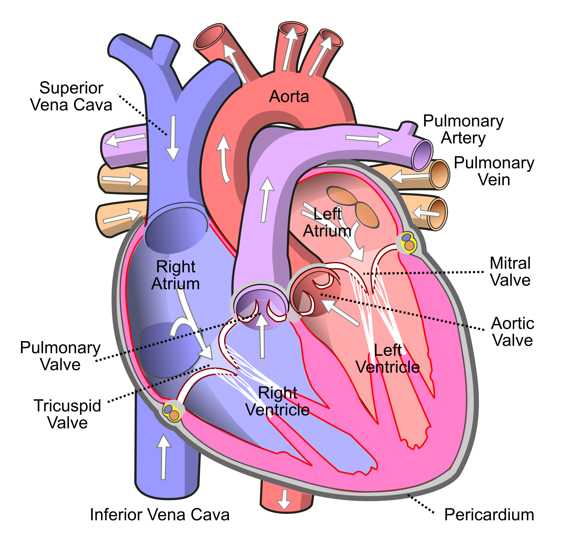
Representation of the heart

2 Data

We first import the peptides.txt file. This is the file that contains your peptide-level intensities. For a MaxQuant search [6], this peptides.txt file can be found by default in the “path_to_raw_files/combined/txt/” folder from the MaxQuant output, with “path_to_raw_files” the folder where raw files were saved. In this tutorial, we will use a MaxQuant peptides file from MaxQuant that can be found in the data tree of the SGA2020 github repository https://github.com/statOmics/SGA2020/tree/data/quantification/heart .

2.1 Data import

Click to see background and code

To import the data we use the QFeatures package.

We generate the object peptideRawFile with the path to the peptideRaws.txt file. Using the grepEcols function, we find the columns that contain the expression data of the peptideRaws in the peptideRaws.txt file.

library(tidyverse)
library(limma)
library(QFeatures)
library(msqrob2)
library(plotly)

peptidesFile <- "https://raw.githubusercontent.com/statOmics/PDA21/data/quantification/heart/peptides.txt"

ecols <- grep("Intensity\\.", names(read.delim(peptidesFile)))

pe <- readQFeatures(
  table = peptidesFile,
  fnames = 1,
  ecol = ecols,
  name = "peptideRaw", sep="\t")

pe

## An instance of class QFeatures containing 1 assays:
##  [1] peptideRaw: SummarizedExperiment with 31319 rows and 12 columns

pe[["peptideRaw"]]

## class: SummarizedExperiment 
## dim: 31319 12 
## metadata(0):
## assays(1): ''
## rownames(31319): AAAAAAAAAK AAAAAAAAEQQSSNGPVK ... YYTPVPCESATAK
##   YYTYLIMNK
## rowData names(91): Sequence N.term.cleavage.window ...
##   Oxidation..M..site.IDs MS.MS.Count
## colnames(12): Intensity.LA3 Intensity.LA4 ... Intensity.RV4
##   Intensity.RV8
## colData names(0):

We will make use from data wrangling functionalities from the tidyverse package. The %>% operator allows us to pipe the output of one function to the next function.

colData(pe)$location <- substr(
  colnames(pe[["peptideRaw"]]),
  11,
  11) %>%
  unlist %>%  
  as.factor

colData(pe)$tissue <- substr(
    colnames(pe[["peptideRaw"]]),
    12,
    12) %>%
    unlist %>%  
    as.factor

colData(pe)$patient <- substr(
  colnames(pe[["peptideRaw"]]),
  13,
  13) %>%
  unlist %>%  
  as.factor

We calculate how many non zero intensities we have per peptide and this will be useful for filtering.

rowData(pe[["peptideRaw"]])$nNonZero <- rowSums(assay(pe[["peptideRaw"]]) > 0)

Peptides with zero intensities are missing peptides and should be represent with a NA value rather than 0.

pe <- zeroIsNA(pe, "peptideRaw") # convert 0 to NA

2.2 Data exploration

Click to see background and code

63% of all peptide intensities are missing and for some peptides we do not even measure a signal in any sample. The missingness is similar across samples.

3 Preprocessing

Click to see background and code

This section preforms standard preprocessing for the peptide data. This include log transformation, filtering and summarisation of the data.

3.1 Log transform the data

pe <- logTransform(pe, base = 2, i = "peptideRaw", name = "peptideLog")
limma::plotDensities(assay(pe[["peptideLog"]]))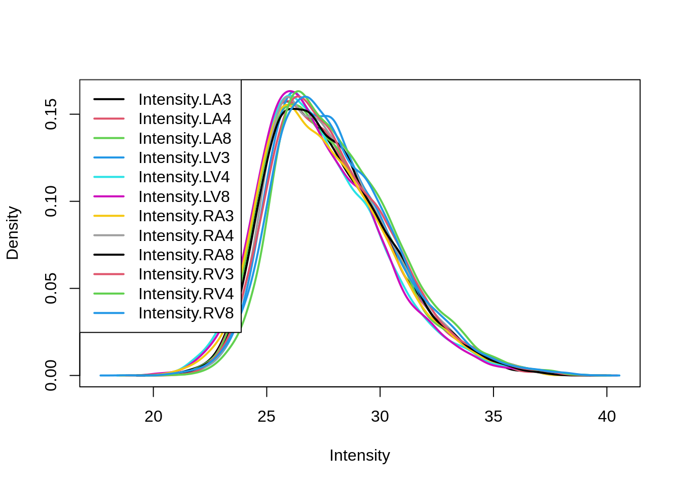

3.2 Filtering

Click to see background and code

3.2.1 Handling overlapping protein groups

In our approach a peptide can map to multiple proteins, as long as there is none of these proteins present in a smaller subgroup.

pe <- filterFeatures(pe, ~ Proteins %in% smallestUniqueGroups(rowData(pe[["peptideLog"]])$Proteins))

3.2.2 Remove reverse sequences (decoys) and contaminants

We now remove the contaminants, peptides that map to decoy sequences, and proteins which were only identified by peptides with modifications.

First look to the names of the variables for the peptide features

pe[["peptideLog"]] %>%
  rowData %>%
  names

##  [1] "Sequence"                "N.term.cleavage.window" 
##  [3] "C.term.cleavage.window"  "Amino.acid.before"      
##  [5] "First.amino.acid"        "Second.amino.acid"      
##  [7] "Second.last.amino.acid"  "Last.amino.acid"        
##  [9] "Amino.acid.after"        "A.Count"                
## [11] "R.Count"                 "N.Count"                
## [13] "D.Count"                 "C.Count"                
## [15] "Q.Count"                 "E.Count"                
## [17] "G.Count"                 "H.Count"                
## [19] "I.Count"                 "L.Count"                
## [21] "K.Count"                 "M.Count"                
## [23] "F.Count"                 "P.Count"                
## [25] "S.Count"                 "T.Count"                
## [27] "W.Count"                 "Y.Count"                
## [29] "V.Count"                 "U.Count"                
## [31] "O.Count"                 "Length"                 
## [33] "Missed.cleavages"        "Mass"                   
## [35] "Proteins"                "Leading.razor.protein"  
## [37] "Start.position"          "End.position"           
## [39] "Gene.names"              "Protein.names"          
## [41] "Unique..Groups."         "Unique..Proteins."      
## [43] "Charges"                 "PEP"                    
## [45] "Score"                   "Identification.type.LA3"
## [47] "Identification.type.LA4" "Identification.type.LA8"
## [49] "Identification.type.LV3" "Identification.type.LV4"
## [51] "Identification.type.LV8" "Identification.type.RA3"
## [53] "Identification.type.RA4" "Identification.type.RA8"
## [55] "Identification.type.RV3" "Identification.type.RV4"
## [57] "Identification.type.RV8" "Fraction.Average"       
## [59] "Fraction.Std..Dev."      "Fraction.1"             
## [61] "Fraction.2"              "Fraction.3"             
## [63] "Fraction.4"              "Fraction.5"             
## [65] "Fraction.6"              "Fraction.7"             
## [67] "Fraction.8"              "Fraction.100"           
## [69] "Experiment.LA3"          "Experiment.LA4"         
## [71] "Experiment.LA8"          "Experiment.LV3"         
## [73] "Experiment.LV4"          "Experiment.LV8"         
## [75] "Experiment.RA3"          "Experiment.RA4"         
## [77] "Experiment.RA8"          "Experiment.RV3"         
## [79] "Experiment.RV4"          "Experiment.RV8"         
## [81] "Intensity"               "Reverse"                
## [83] "Potential.contaminant"   "id"                     
## [85] "Protein.group.IDs"       "Mod..peptide.IDs"       
## [87] "Evidence.IDs"            "MS.MS.IDs"              
## [89] "Best.MS.MS"              "Oxidation..M..site.IDs" 
## [91] "MS.MS.Count"             "nNonZero"

No information on decoys.

pe <- filterFeatures(pe,~ Potential.contaminant != "+")

3.2.3 Drop peptides that were only identified in one sample

We keep peptides that were observed at least twice.

pe <- filterFeatures(pe,~nNonZero >= 2)
nrow(pe[["peptideLog"]])

## [1] 17432

We keep 17432 peptides after filtering.

3.3 Normalize the data

Click to see background and code

pe <- normalize(pe, 
                i = "peptideLog", 
                name = "peptideNorm", 
                method = "center.median")

3.3.1 Explore normalized data

Click to see background and code

After normalisation the density curves for all samples are comparable.

limma::plotDensities(assay(pe[["peptideNorm"]]))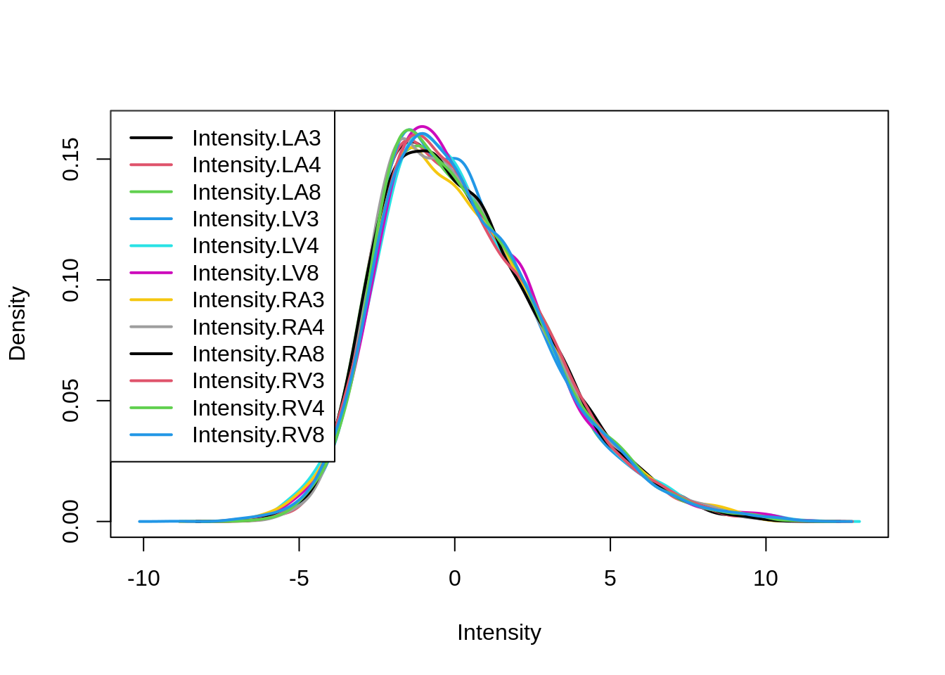

This is more clearly seen is a boxplot.

boxplot(assay(pe[["peptideNorm"]]), col = palette()[-1],
       main = "Peptide distribtutions after normalisation", ylab = "intensity")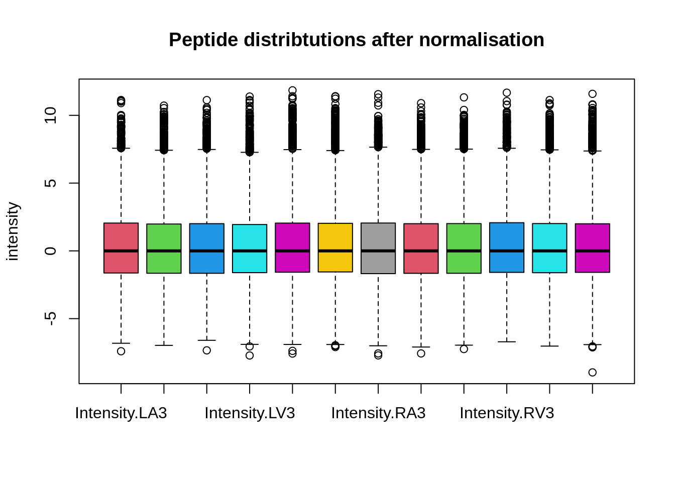

We can visualize our data using a Multi Dimensional Scaling plot, eg. as provided by the limma package.

limma::plotMDS(assay(pe[["peptideNorm"]]),
  col = colData(pe)$location:colData(pe)$tissue %>%
    as.numeric,
  labels = colData(pe) %>%
    rownames %>%  
    substr(start = 11, stop = 13)
  )

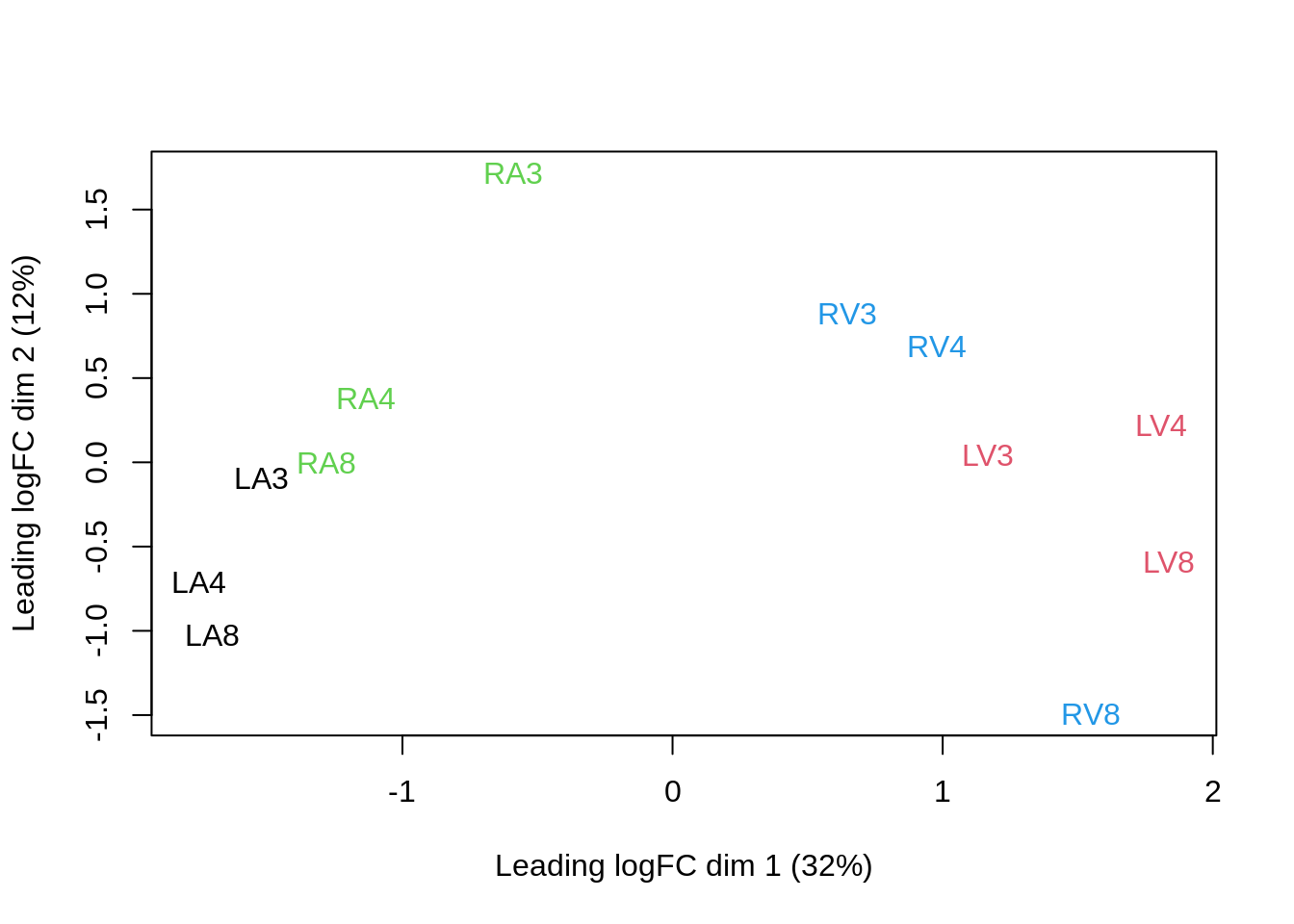
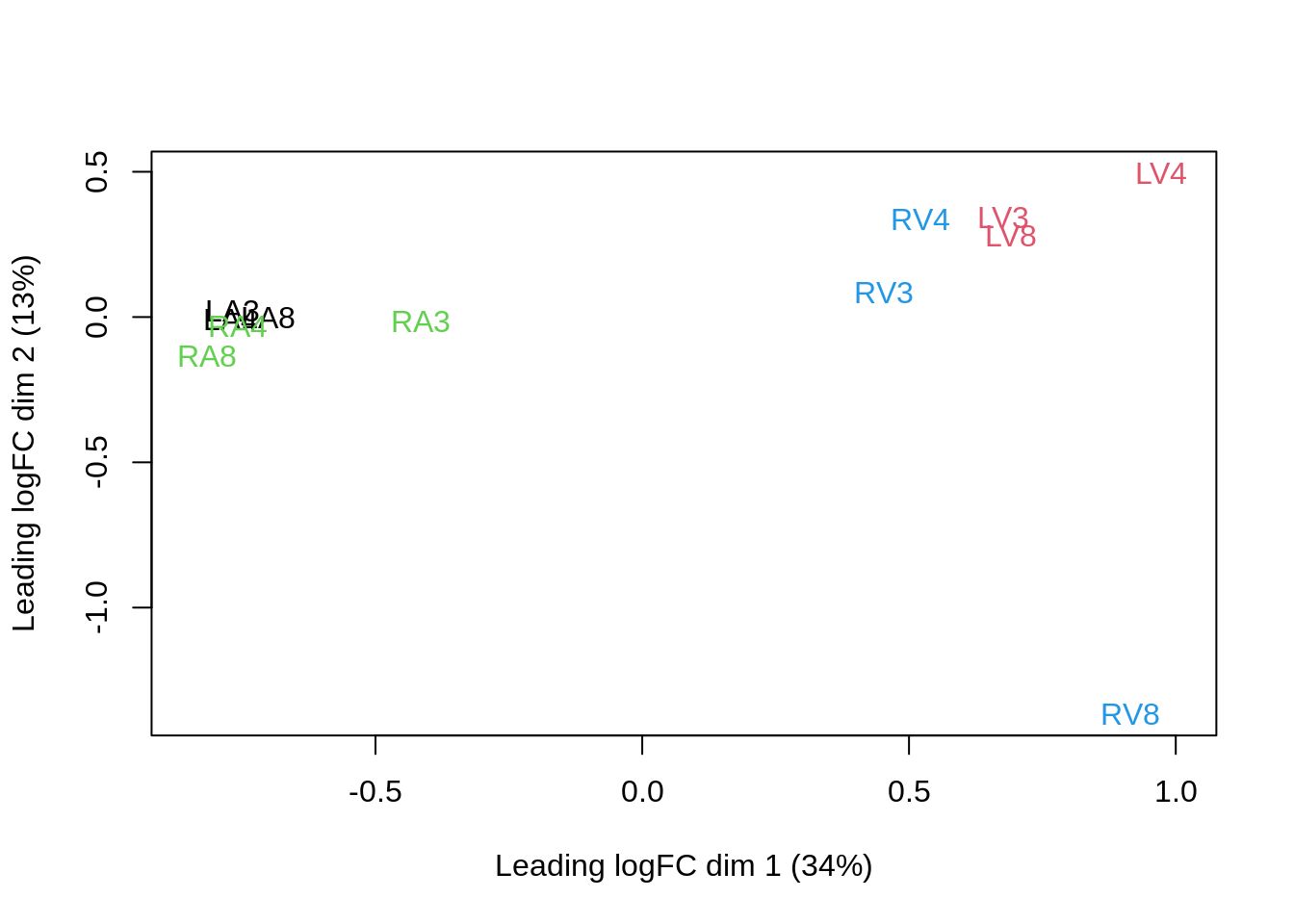
The first axis in the plot is showing the leading log fold changes (differences on the log scale) between the samples.

3.4 Summarization to protein level

Click to see background and code

We use robust summarization in aggregateFeatures. This is the default workflow of aggregateFeatures so you do not have to specifiy the argument fun. However, because we compare methods we have included the fun argument to show the summarization method explicitely.

pe <- aggregateFeatures(pe,
 i = "peptideNorm",
 fcol = "Proteins",
 na.rm = TRUE,
 name = "proteinRobust",
 fun = MsCoreUtils::robustSummary)

## Your quantitative and row data contain missing values. Please read the
## relevant section(s) in the aggregateFeatures manual page regarding the
## effects of missing values on data aggregation.

plotMDS(assay(pe[["proteinRobust"]]),
  col = colData(pe)$location:colData(pe)$tissue %>%
    as.numeric,
  labels = colData(pe) %>%
    rownames %>%  
    substr(start = 11, stop = 13)
)

4 Data Analysis

4.1 Estimation

We model the protein level expression values using msqrob. By default msqrob2 estimates the model parameters using robust regression.

pe <- msqrob(
  object = pe,
  i = "proteinRobust",
  formula = ~ location*tissue + patient)

4.2 Inference

Explore Design

library(ExploreModelMatrix)
VisualizeDesign(colData(pe),~ location*tissue + patient)$plotlist

## $`location = L`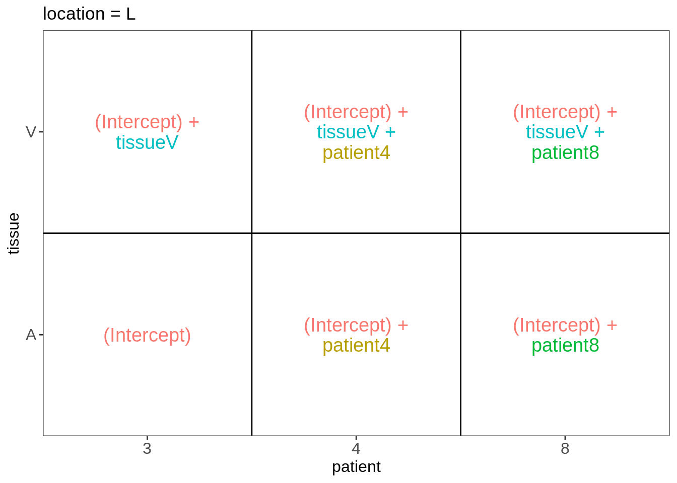

## 
## $`location = R`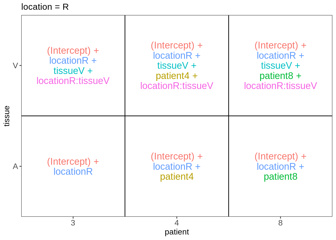

design <- model.matrix(~location*tissue + patient, data = colData(pe))
L <- makeContrast(
  c(
    "tissueV = 0",
    "tissueV + locationR:tissueV = 0",
    "tissueV + 0.5*locationR:tissueV = 0","locationR:tissueV = 0"),
  parameterNames = colnames(design)
  )


pe <- hypothesisTest(object = pe, i = "proteinRobust", contrast = L, overwrite=TRUE)

4.3 Evaluate results contrast \(\log_2 FC_{V-A}^L\)

4.3.1 Volcano-plot

volcanoLeft <- ggplot(rowData(pe[["proteinRobust"]])$"tissueV",
                 aes(x = logFC, y = -log10(pval), color = adjPval < 0.05)) +
 geom_point(cex = 2.5) +
 scale_color_manual(values = alpha(c("black", "red"), 0.5)) + theme_minimal()
volcanoLeft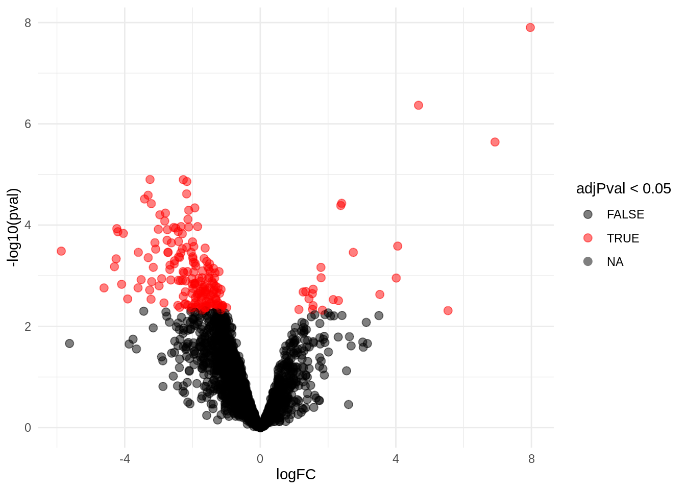

4.3.2 Heatmap

We first select the names of the proteins that were declared signficant.

sigNamesLeft <- rowData(pe[["proteinRobust"]])$tissueV %>%
 rownames_to_column("proteinRobust") %>%
 filter(adjPval<0.05) %>%
 pull(proteinRobust)
heatmap(assay(pe[["proteinRobust"]])[sigNamesLeft, ])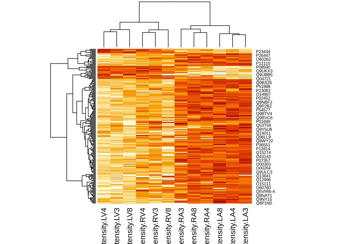

There are 199 proteins significantly differentially expressed at the 5% FDR level.

rowData(pe[["proteinRobust"]])$tissueV %>%
  cbind(.,rowData(pe[["proteinRobust"]])$Protein.names) %>%
  na.exclude %>%
  filter(adjPval<0.05) %>%
  arrange(pval)  %>%
  head(10) %>%
  knitr::kable(.) 

	logFC	se	df	t	pval	adjPval	rowData(pe[[“proteinRobust”]])$Protein.names
P08590	7.967951	0.4374873	9.367147	18.212987	0.00e+00	0.0000254	Myosin light chain 3
P12883	4.669883	0.3716628	9.181668	12.564838	4.00e-07	0.0004379	Myosin-7
P10916	6.926109	0.5291456	7.367147	13.089231	2.30e-06	0.0015506	Myosin regulatory light chain 2, ventricular/cardiac muscle isoform
Q6UWY5	-3.253643	0.3828898	9.113260	-8.497596	1.26e-05	0.0046705	Olfactomedin-like protein 1
O75368	-2.271594	0.2715292	9.289260	-8.365932	1.27e-05	0.0046705	SH3 domain-binding glutamic acid-rich-like protein
P46821	-2.166880	0.2632626	9.367147	-8.230871	1.38e-05	0.0046705	Microtubule-associated protein 1B;MAP1B heavy chain;MAP1 light chain LC1
O95865	-2.173219	0.2826203	9.367147	-7.689536	2.42e-05	0.0065478	N(G),N(G)-dimethylarginine dimethylaminohydrolase 2
Q8N474	-3.309023	0.3804443	7.897481	-8.697787	2.58e-05	0.0065478	Secreted frizzled-related protein 1
Q9ULL5-3	-3.416540	0.3998973	7.846127	-8.543546	3.05e-05	0.0068882	Proline-rich protein 12
P14854	2.401913	0.3057866	8.431469	7.854864	3.71e-05	0.0069621	Cytochrome c oxidase subunit 6B1

4.4 Evaluate results contrast \(\log_2 FC_{V-A}^R\)

4.4.1 Volcano-plot

volcanoRight <- ggplot(rowData(pe[["proteinRobust"]])$"tissueV + locationR:tissueV",
                 aes(x = logFC, y = -log10(pval), color = adjPval < 0.05)) +
 geom_point(cex = 2.5) +
 scale_color_manual(values = alpha(c("black", "red"), 0.5)) + theme_minimal()
volcanoRight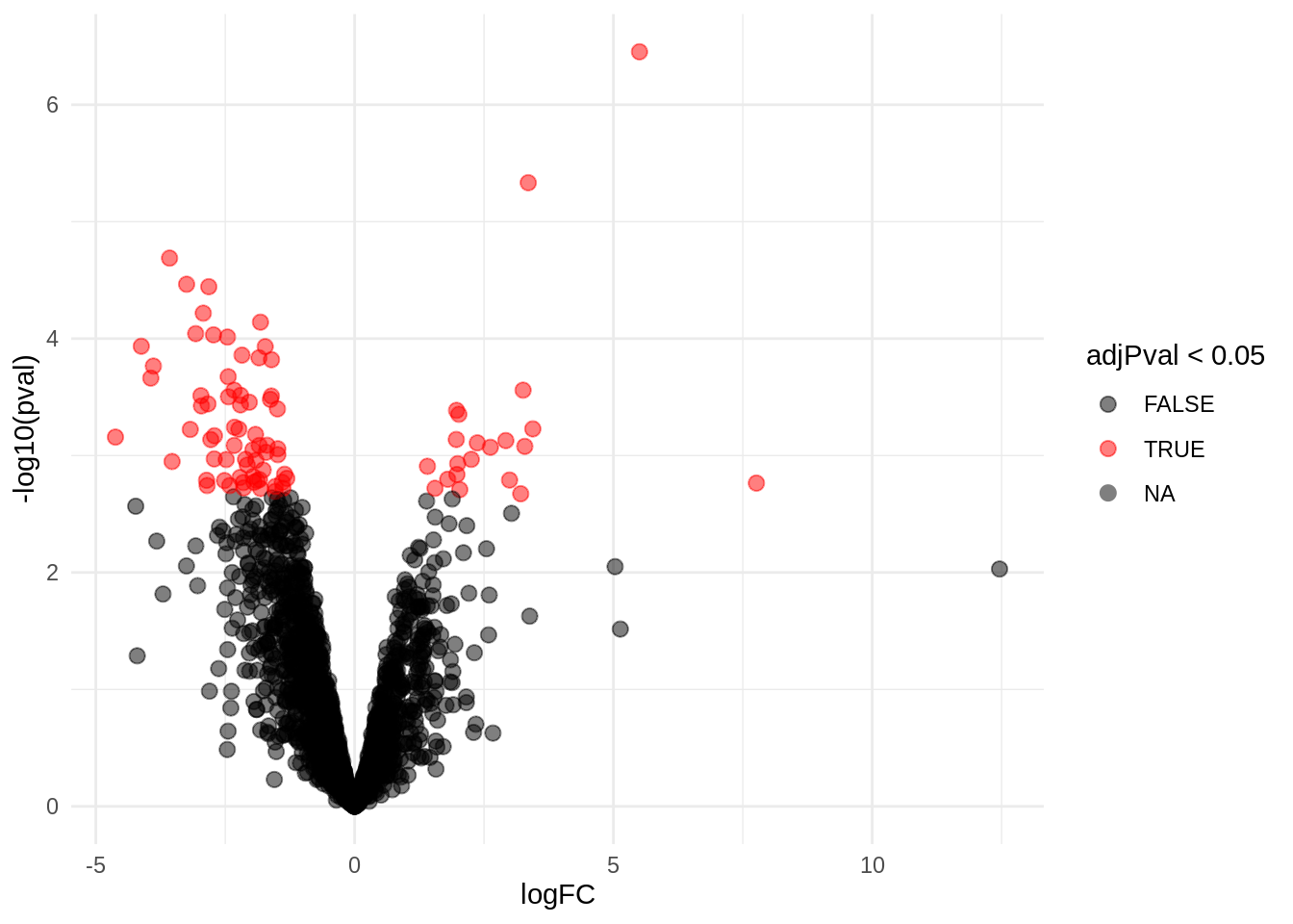

4.4.2 Heatmap

We first select the names of the proteins that were declared signficant.

sigNamesRight <- rowData(pe[["proteinRobust"]])$"tissueV + locationR:tissueV" %>%
 rownames_to_column("proteinRobust") %>%
 filter(adjPval<0.05) %>%
 pull(proteinRobust)
heatmap(assay(pe[["proteinRobust"]])[sigNamesRight, ])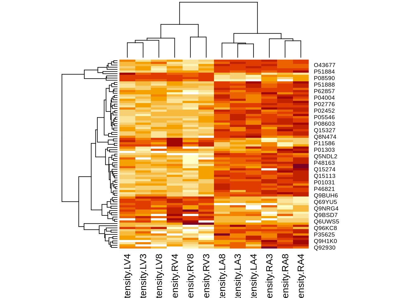

There are 87 proteins significantly differentially expressed at the 5% FDR level.

rowData(pe[["proteinRobust"]])$"tissueV + locationR:tissueV"  %>%
  cbind(.,rowData(pe[["proteinRobust"]])$Protein.names) %>%
  na.exclude %>%
  filter(adjPval<0.05) %>%
  arrange(pval) %>%
  head(10) %>%
  knitr::kable(.)

	logFC	se	df	t	pval	adjPval	rowData(pe[[“proteinRobust”]])$Protein.names
P08590	5.503838	0.4374873	9.367147	12.580565	4.00e-07	0.0007167	Myosin light chain 3
P06858	3.354674	0.3544630	9.249267	9.464102	4.60e-06	0.0047205	Lipoprotein lipase
Q9ULD0	-3.575906	0.3737222	7.367147	-9.568355	2.05e-05	0.0138839	2-oxoglutarate dehydrogenase-like, mitochondrial
P35442	-3.246460	0.4065828	8.367147	-7.984746	3.43e-05	0.0146265	Thrombospondin-2
P02776	-2.818363	0.3421511	7.975973	-8.237189	3.60e-05	0.0146265	Platelet factor 4;Platelet factor 4, short form
P21810	-2.924783	0.4081159	8.756796	-7.166550	6.06e-05	0.0197128	Biglycan
O75368	-1.819326	0.2697137	9.289260	-6.745396	7.23e-05	0.0197128	SH3 domain-binding glutamic acid-rich-like protein
A6NMZ7	-3.070848	0.4709254	9.367147	-6.520879	9.07e-05	0.0197128	Collagen alpha-6(VI) chain
P54652	-2.726681	0.4117048	9.078544	-6.622904	9.29e-05	0.0197128	Heat shock-related 70 kDa protein 2
Q6UWY5	-2.456874	0.3739352	9.113260	-6.570320	9.70e-05	0.0197128	Olfactomedin-like protein 1

4.5 Evaluate results average contrast \(\log_2 FC_{V-A}\)

4.5.1 Volcano-plot

volcanoAvg <- ggplot(rowData(pe[["proteinRobust"]])$"tissueV + 0.5 * locationR:tissueV",
                 aes(x = logFC, y = -log10(pval), color = adjPval < 0.05)) +
 geom_point(cex = 2.5) +
 scale_color_manual(values = alpha(c("black", "red"), 0.5)) + theme_minimal()
volcanoAvg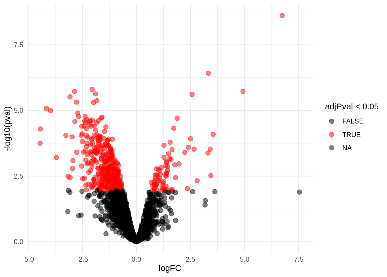

4.5.2 Heatmap

We first select the names of the proteins that were declared signficant.

sigNamesAvg <- rowData(pe[["proteinRobust"]])$"tissueV + 0.5 * locationR:tissueV" %>%
 rownames_to_column("proteinRobust") %>%
 filter(adjPval<0.05) %>%
 pull(proteinRobust)
heatmap(assay(pe[["proteinRobust"]])[sigNamesAvg, ])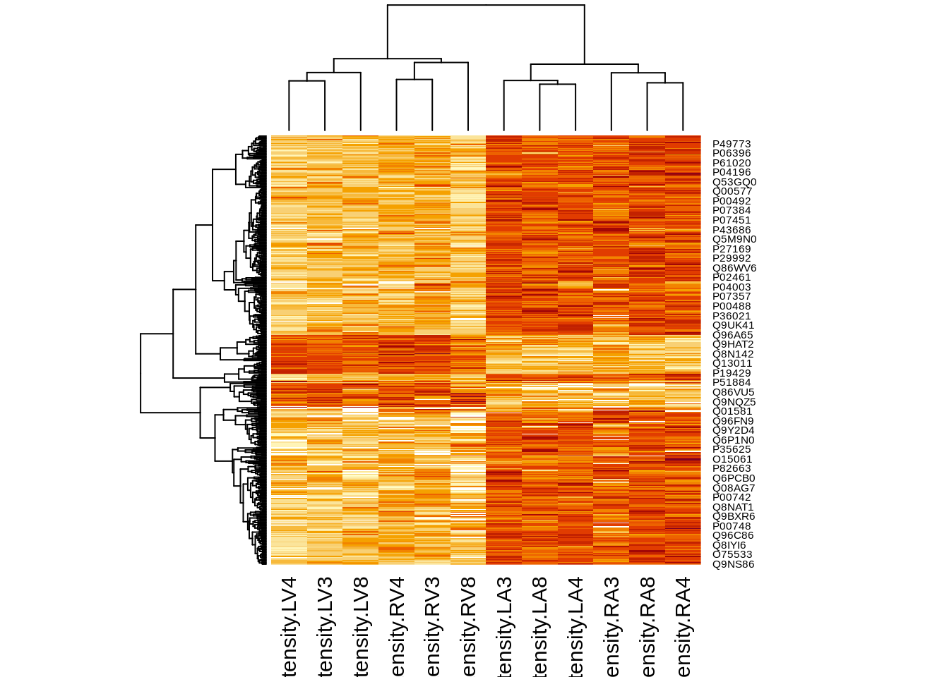

There are 449 proteins significantly differentially expressed at the 5% FDR level.

rowData(pe[["proteinRobust"]])$"tissueV + 0.5 * locationR:tissueV" %>%
  cbind(.,rowData(pe[["proteinRobust"]])$Protein.names) %>%
  na.exclude %>%
  filter(adjPval<0.05) %>%
  arrange(pval) %>%
  head(10) %>%
  knitr::kable(.) 

	logFC	se	df	t	pval	adjPval	rowData(pe[[“proteinRobust”]])$Protein.names
P08590	6.735894	0.3093503	9.367147	21.77433	0.0e+00	0.0000049	Myosin light chain 3
P12883	3.319491	0.2606314	9.181668	12.73634	4.0e-07	0.0003891	Myosin-7
O75368	-2.045460	0.1913593	9.289260	-10.68911	1.6e-06	0.0007082	SH3 domain-binding glutamic acid-rich-like protein
Q6UWY5	-2.855258	0.2675968	9.113260	-10.67000	1.9e-06	0.0007082	Olfactomedin-like protein 1
P10916	4.923642	0.3661150	7.367147	13.44835	1.9e-06	0.0007082	Myosin regulatory light chain 2, ventricular/cardiac muscle isoform
P46821	-1.886709	0.1861547	9.367147	-10.13517	2.4e-06	0.0007082	Microtubule-associated protein 1B;MAP1B heavy chain;MAP1 light chain LC1
P06858	2.571933	0.2519480	9.249267	10.20819	2.4e-06	0.0007082	Lipoprotein lipase
P21810	-3.069662	0.2931217	8.756796	-10.47231	3.0e-06	0.0007662	Biglycan
P05546	-1.829841	0.1916993	9.271661	-9.54537	4.2e-06	0.0009134	Heparin cofactor 2
P35442	-2.773755	0.2689292	8.367147	-10.31407	4.8e-06	0.0009134	Thrombospondin-2

4.6 Interaction

4.6.1 Volcano-plot

volcanoInt <- ggplot(rowData(pe[["proteinRobust"]])$"locationR:tissueV",
                 aes(x = logFC, y = -log10(pval), color = adjPval < 0.05)) +
 geom_point(cex = 2.5) +
 scale_color_manual(values = alpha(c("black", "red"), 0.5)) + theme_minimal()
volcanoInt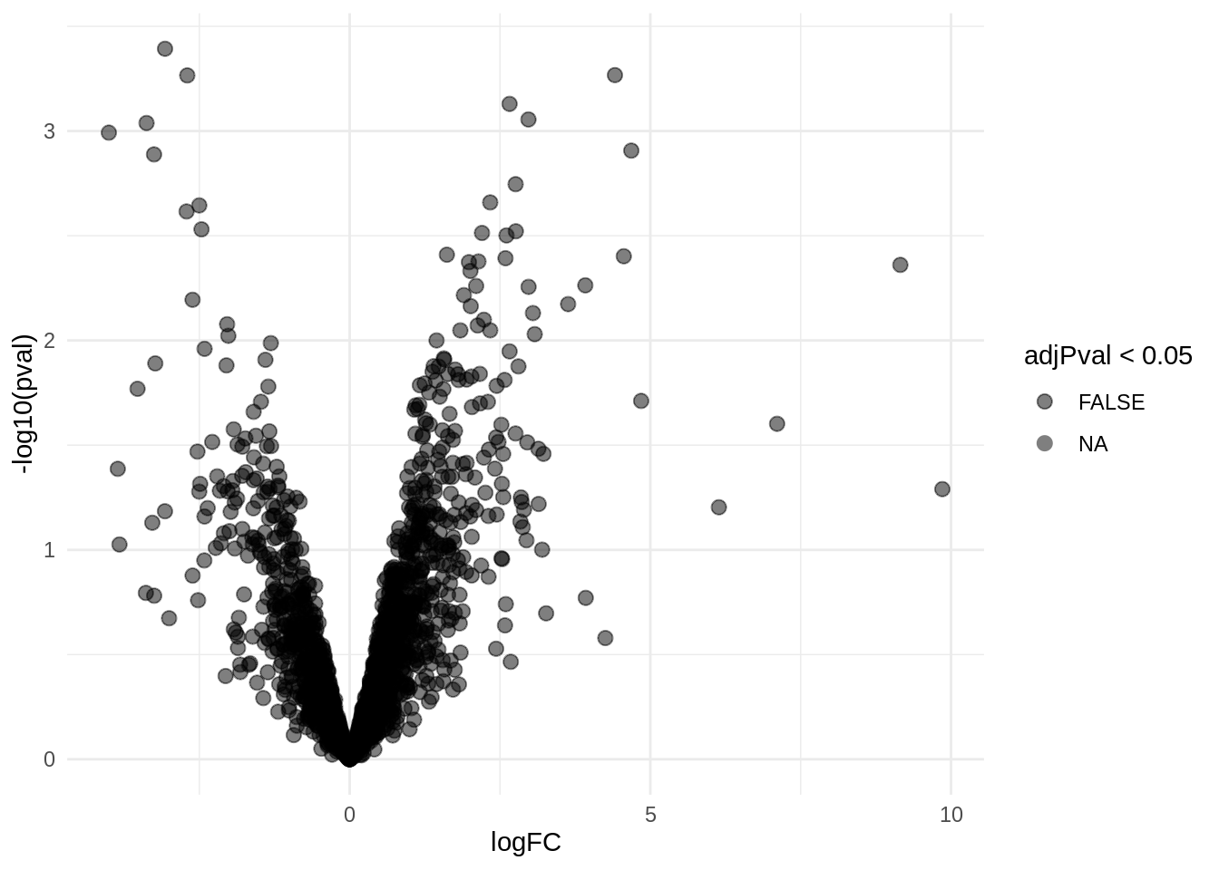

4.6.2 Heatmap

There were no genes significant at the 5% FDR level. We return the top 25 genes.

sigNamesInt <- rowData(pe[["proteinRobust"]])$"locationR:tissueV" %>%
 rownames_to_column("proteinRobust") %>%
 filter(adjPval<0.05) %>%
 pull(proteinRobust)
hlp <- order((rowData(pe[["proteinRobust"]])$"locationR:tissueV")[,"adjPval"])[1:25]
heatmap(assay(pe[["proteinRobust"]])[hlp, ])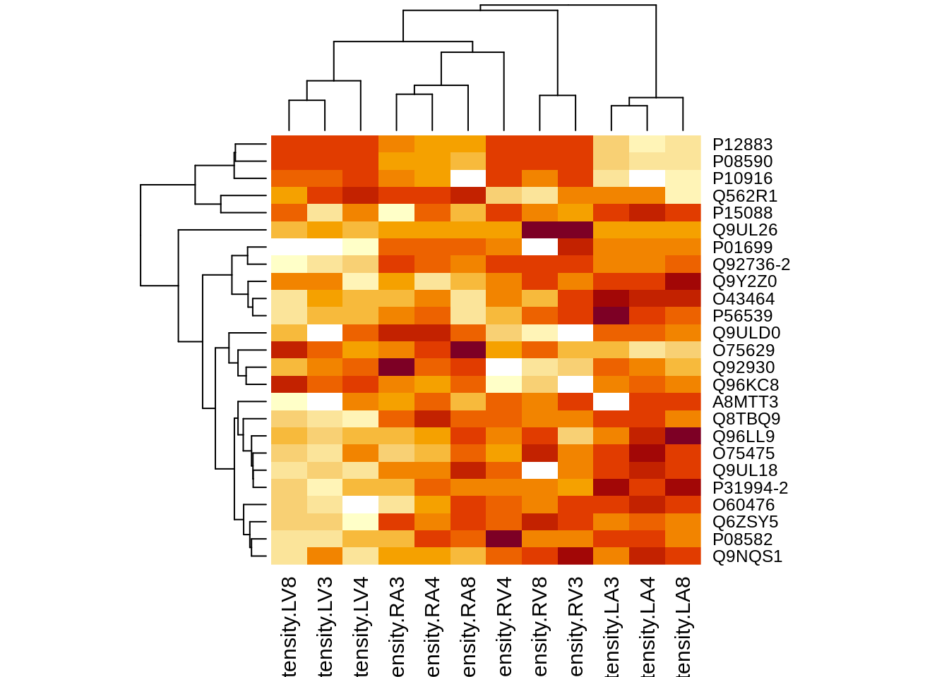

There are 0 proteins significantly differentially expressed at the 5% FDR level.

rowData(pe[["proteinRobust"]])$"locationR:tissueV" %>%
  cbind(.,rowData(pe[["proteinRobust"]])$Protein.names) %>%
  na.exclude %>%
  filter(adjPval<0.05) %>%
  head(10) %>%
  knitr::kable(.) 

logFC	se	df	t	pval	adjPval	rowData(pe[[“proteinRobust”]])$Protein.names

---

This work is licensed under the CC BY-SA-4.0 licence.