EuroBioc demo: Analysis of the CPTAC Spike-in Study

1 The CPTAC Spike-In Study

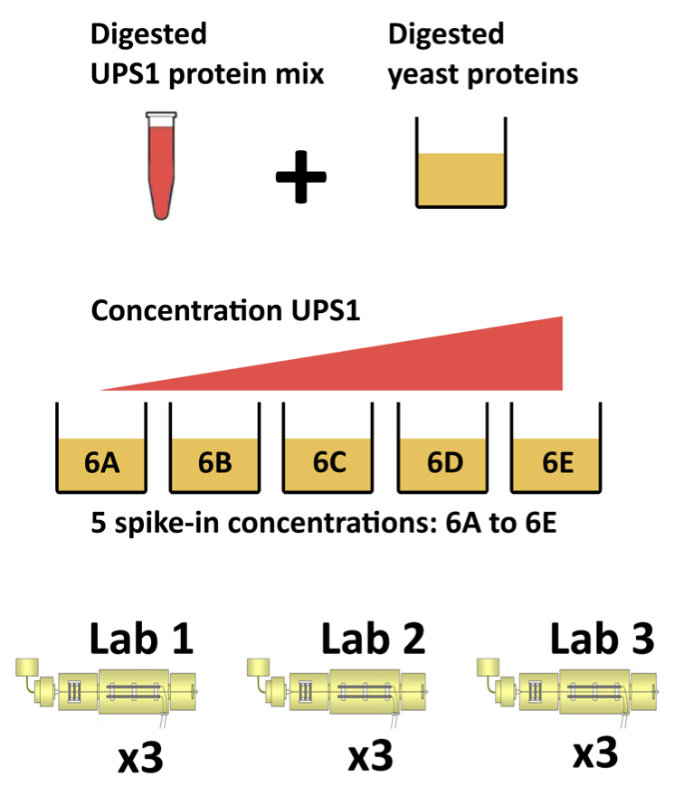
This case-study is a subset of the data of the 6th study of the Clinical Proteomic Technology Assessment for Cancer (CPTAC) [5]. In this experiment, the authors spiked the Sigma Universal Protein Standard mixture 1 (UPS1) containing 48 different human proteins in a protein background of 60 ng/\(\mu\)L Saccharomyces cerevisiae strain BY4741.

Five different spike-in concentrations were used:

• 6A: 0.25 fmol UPS1 proteins/\(\mu L\),
• 6B: 0.74 fmol UPS1 proteins/\(\mu L\),
• 6C: 2.22 fmol UPS1 proteins/\(\mu L\),
• 6D: 6.67 fmol UPS1 proteins/\(\mu L\) and
• 6E: 20 fmol UPS1 proteins/\(\mu L\)).

The data were searched with MaxQuant version 1.5.2.8, and detailed search settings were described in Goeminne et al. (2016) [1]. Three replicates are available for each concentration.

2 QFeatures: data infrastructure

We will use the QFeatures package that provides the infrastructure to store, process, manipulate and analyse quantitative data/features from mass spectrometry experiments. It is based on the SummarizedExperiment and MultiAssayExperiment classes.

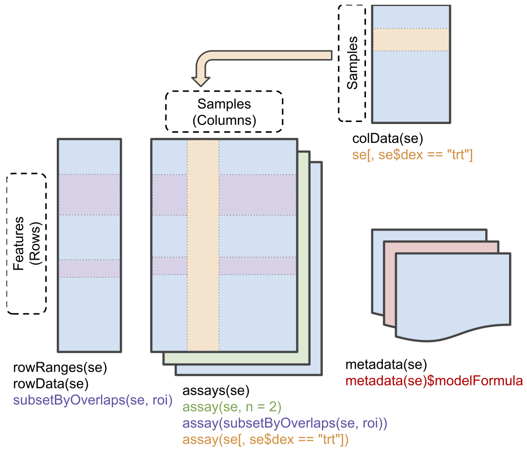
Conceptual representation of a SummarizedExperiment object. Assays contain information on the measured omics features (rows) for different samples (columns). The rowData contains information on the omics features, the colData contains information on the samples, i.e. experimental design etc.

Assays in a QFeatures object have a hierarchical relation:

• proteins are composed of peptides,
• themselves produced by peptide spectrum matches
• relations between assays are tracked and recorded throughout data processing

Conceptual representation of a QFeatures object and the aggregative relation between different assays. Image from the QFeatures vignette.

3 Data preparation

Let’s start by loading the packages that we will need

library(tidyverse)
library(limma)
library(QFeatures)
library(msqrob2)

3.1 Import data from the CPTAC study

1. We use MS-data quantified with MaxQuant that contains MS1 intensities summarized at the peptide level. This file contains a subset of the data and is available in the msdata package.

(basename(f <- msdata::quant(full.names = TRUE)))

## [1] "cptac_a_b_peptides.txt"

2. Maxquant stores the intensity data for the different samples in columnns that start with “Intensity”. We can retreive the column names with the intensity data with the code below:

grep("Intensity\\.", names(read.delim(f)), value = TRUE)

## [1] "Intensity.6A_7" "Intensity.6A_8" "Intensity.6A_9" "Intensity.6B_7"
## [5] "Intensity.6B_8" "Intensity.6B_9"

(ecols <- grep("Intensity\\.", names(read.delim(f))))

## [1] 56 57 58 59 60 61

3. Read the data and store it in QFeatures object

qf <- readQFeatures(
    f, fnames = 1, ecol = ecols,
    name = "peptideRaw", sep = "\t")

The QFeatures object qf currently contains a single assay, named peptideRaw, composed of 11466 peptides measured in 6 samples.

qf

## An instance of class QFeatures containing 1 assays:
##  [1] peptideRaw: SummarizedExperiment with 11466 rows and 6 columns

We can access the unique assay by index (i.e. 1) or by name (i.e “peptideRaw”) using the [[]] operator, which returns an instance of class SummarizedExperiment:

qf[[1]]

## class: SummarizedExperiment 
## dim: 11466 6 
## metadata(0):
## assays(1): ''
## rownames(11466): AAAAGAGGAGDSGDAVTK AAAALAGGK ... YYTVFDRDNNR
##   YYTVFDRDNNRVGFAEAAR
## rowData names(65): Sequence N.term.cleavage.window ...
##   Oxidation..M..site.IDs MS.MS.Count
## colnames(6): Intensity.6A_7 Intensity.6A_8 ... Intensity.6B_8
##   Intensity.6B_9
## colData names(0):

qf[["peptideRaw"]]

## class: SummarizedExperiment 
## dim: 11466 6 
## metadata(0):
## assays(1): ''
## rownames(11466): AAAAGAGGAGDSGDAVTK AAAALAGGK ... YYTVFDRDNNR
##   YYTVFDRDNNRVGFAEAAR
## rowData names(65): Sequence N.term.cleavage.window ...
##   Oxidation..M..site.IDs MS.MS.Count
## colnames(6): Intensity.6A_7 Intensity.6A_8 ... Intensity.6B_8
##   Intensity.6B_9
## colData names(0):

The quantitative data can be accessed with the assay() function

assay(qf[[1]])[1:10, 1:3]

##                           Intensity.6A_7 Intensity.6A_8 Intensity.6A_9
## AAAAGAGGAGDSGDAVTK                     0              0          66760
## AAAALAGGK                        2441300        1220000        1337600
## AAAALAGGKK                       1029200         668040         638990
## AAADALSDLEIK                      515460         670780         712140
## AAADALSDLEIKDSK                   331130         420900         365560
## AAAEEFQR                               0              0          51558
## AAAEGPMK                               0              0              0
## AAAEGVANLHLDEATGEMVSK                  0              0              0
## AAAEYEKGEYETAISTLNDAVEQGR              0              0              0
## AAAHSSLK                               0              0              0

3.2 Explore object

• The rowData contains information on the features (peptides) in the assay. E.g. Sequence, protein, …

rowData(qf[["peptideRaw"]])[, c("Proteins", "Sequence", "Charges")]

## DataFrame with 11466 rows and 3 columns
##                          Proteins      Sequence     Charges
##                       <character>   <character> <character>
## AAAAGAGGAGDSGDAVTK  sp|P38915|... AAAAGAGGAG...           2
## AAAALAGGK           sp|Q3E792|...     AAAALAGGK           2
## AAAALAGGKK          sp|Q3E792|...    AAAALAGGKK           2
## AAADALSDLEIK        sp|P09938|... AAADALSDLE...           2
## AAADALSDLEIKDSK     sp|P09938|... AAADALSDLE...           3
## ...                           ...           ...         ...
## YYSIYDLGNNAVGLAK    sp|P07267|... YYSIYDLGNN...           2
## YYTFNGPNYNENETIR    sp|Q00955|... YYTFNGPNYN...           2
## YYTITEVATR          sp|P38891|...    YYTITEVATR           2
## YYTVFDRDNNR         P07339ups|... YYTVFDRDNN...           2
## YYTVFDRDNNRVGFAEAAR P07339ups|... YYTVFDRDNN...           3

• The colData contains information on the samples, but is currently empty:

colData(qf)

## DataFrame with 6 rows and 0 columns

• We can rename the primary sample names and assay column names

colnames(qf)[[1]]

## [1] "Intensity.6A_7" "Intensity.6A_8" "Intensity.6A_9" "Intensity.6B_7"
## [5] "Intensity.6B_8" "Intensity.6B_9"

(new_names <- sub("Intensity\\.", "", colnames(qf)[[1]]))

## [1] "6A_7" "6A_8" "6A_9" "6B_7" "6B_8" "6B_9"

qf <- renameColname(qf, i = 1, new_names) |>
  renamePrimary(new_names)

• We should also update the colData with information on the design

qf$lab <- rep("lab3", 6)
qf$condition <- factor(rep(c("A", "B"), each = 3))
qf$spikeConcentration <- rep(c(A = 0.25, B = 0.74),
                             each = 3)

colData(qf)

## DataFrame with 6 rows and 3 columns
##              lab condition spikeConcentration
##      <character>  <factor>          <numeric>
## 6A_7        lab3         A               0.25
## 6A_8        lab3         A               0.25
## 6A_9        lab3         A               0.25
## 6B_7        lab3         B               0.74
## 6B_8        lab3         B               0.74
## 6B_9        lab3         B               0.74

3.3 Missingness

Peptides with zero intensities are missing peptides and should be represent with a NA value rather than 0. This can be done with the zeroIsNA() function. We can then use nNA() on the individual assay to compute missingness summaries:

qf <- zeroIsNA(qf, "peptideRaw")
na <- nNA(qf[[1]])
na

## $nNA
## DataFrame with 1 row and 2 columns
##         nNA       pNA
##   <integer> <numeric>
## 1     31130   45.2497
## 
## $nNArows
## DataFrame with 11466 rows and 3 columns
##                name       nNA       pNA
##         <character> <integer> <numeric>
## 1     AAAAGAGGAG...         4   66.6667
## 2         AAAALAGGK         0    0.0000
## 3        AAAALAGGKK         0    0.0000
## 4     AAADALSDLE...         0    0.0000
## 5     AAADALSDLE...         0    0.0000
## ...             ...       ...       ...
## 11462 YYSIYDLGNN...         6  100.0000
## 11463 YYTFNGPNYN...         3   50.0000
## 11464    YYTITEVATR         4   66.6667
## 11465 YYTVFDRDNN...         6  100.0000
## 11466 YYTVFDRDNN...         6  100.0000
## 
## $nNAcols
## DataFrame with 6 rows and 3 columns
##          name       nNA       pNA
##   <character> <integer> <numeric>
## 1        6A_7      4743   41.3658
## 2        6A_8      5483   47.8196
## 3        6A_9      5320   46.3980
## 4        6B_7      4721   41.1739
## 5        6B_8      5563   48.5174
## 6        6B_9      5300   46.2236

• 31130 peptides intensities, corresponding to 45%, are missing and for some peptides we do not even measure a signal in any sample.
• For each sample, the proportion fluctuates between 41.4 and 48.5%.
• The table below shows the number of peptides that have 0, 1, … and up to 6 missing values.

table(na$nNArows$nNA)

## 
##    0    1    2    3    4    5    6 
## 4059  990  884  717  934  807 3075

We will want to keep features that are missing in no more than 2 samples.

rowData(qf[[1]])$keepNA <- na$nNArows$nNA <= 4

4 Preprocessing

This section preforms preprocessing for the peptide data. This include

• log transformation,
• filtering and
• summarisation of the data.

4.1 Log transform the data

qf <- logTransform(qf, base = 2,
                   i = "peptideRaw",
                   name = "peptideLog")
qf

## An instance of class QFeatures containing 2 assays:
##  [1] peptideRaw: SummarizedExperiment with 11466 rows and 6 columns 
##  [2] peptideLog: SummarizedExperiment with 11466 rows and 6 columns

4.2 Filtering

Handling overlapping protein groups: in our approach a peptide can map to multiple proteins, as long as there is none of these proteins present in a smaller subgroup.

sug <- smallestUniqueGroups(rowData(qf[["peptideRaw"]])$Proteins)
filterFeatures(qf, ~ Proteins %in% sug)

## An instance of class QFeatures containing 2 assays:
##  [1] peptideRaw: SummarizedExperiment with 10740 rows and 6 columns 
##  [2] peptideLog: SummarizedExperiment with 10740 rows and 6 columns

Remove reverse sequences (decoys) and contaminants: we now remove the contaminants and peptides that map to decoy sequences.

filterFeatures(qf, ~ Reverse != "+")

## An instance of class QFeatures containing 2 assays:
##  [1] peptideRaw: SummarizedExperiment with 11436 rows and 6 columns 
##  [2] peptideLog: SummarizedExperiment with 11436 rows and 6 columns

filterFeatures(qf, ~ Potential.contaminant != "+")

## An instance of class QFeatures containing 2 assays:
##  [1] peptideRaw: SummarizedExperiment with 11385 rows and 6 columns 
##  [2] peptideLog: SummarizedExperiment with 11385 rows and 6 columns

Drop peptides that were only identified in one sample: we keep peptides that were observed at last twice, i.e. those that have no more that 4 missing values

filterFeatures(qf, ~ keepNA)

## An instance of class QFeatures containing 2 assays:
##  [1] peptideRaw: SummarizedExperiment with 7584 rows and 6 columns 
##  [2] peptideLog: SummarizedExperiment with 7584 rows and 6 columns

Putting it all together:

qf <- qf |>
    filterFeatures(~ Proteins %in% sug) |>
    filterFeatures(~ Reverse != "+") |>
    filterFeatures(~ Potential.contaminant != "+") |>
    filterFeatures(~ keepNA)
qf

## An instance of class QFeatures containing 2 assays:
##  [1] peptideRaw: SummarizedExperiment with 7011 rows and 6 columns 
##  [2] peptideLog: SummarizedExperiment with 7011 rows and 6 columns

We keep 7011 peptides upon filtering.

4.3 Normalisation

We normalise the data by substracting the sample median from every intensity for peptide \(p\) in a sample \(i\):

\[y_{ip}^\text{norm} = y_{ip} - \hat\mu_i\]

with \(\hat\mu_i\) the median intensity over all observed peptides in sample \(i\).

qf <- normalize(qf,
                i = "peptideLog",
                name = "peptideNorm",
                method = "center.median")
qf

## An instance of class QFeatures containing 3 assays:
##  [1] peptideRaw: SummarizedExperiment with 7011 rows and 6 columns 
##  [2] peptideLog: SummarizedExperiment with 7011 rows and 6 columns 
##  [3] peptideNorm: SummarizedExperiment with 7011 rows and 6 columns

4.4 Explore normalized data

Upon the normalisation the density curves follow a similar distribution.

as_tibble(longFormat(qf[, , 2:3], colvars = "condition")) %>%
    ggplot(aes(x = value, group = primary, colour = condition)) +
    geom_density() +
    facet_grid(assay ~ .) +
    theme_bw()

## Warning: 'experiments' dropped; see 'metadata'

## harmonizing input:
##   removing 6 sampleMap rows not in names(experiments)

## Warning: Removed 16334 rows containing non-finite values (stat_density).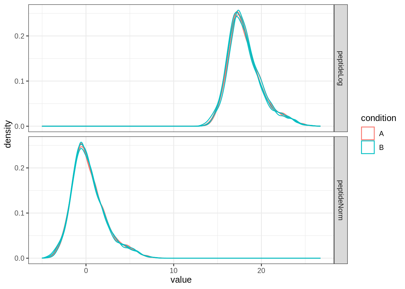

We can visualize our data using a Multi Dimensional Scaling plot, eg. as provided by the limma package.

assay(qf[["peptideNorm"]]) |>
    limma::plotMDS(col = as.numeric(qf$condition))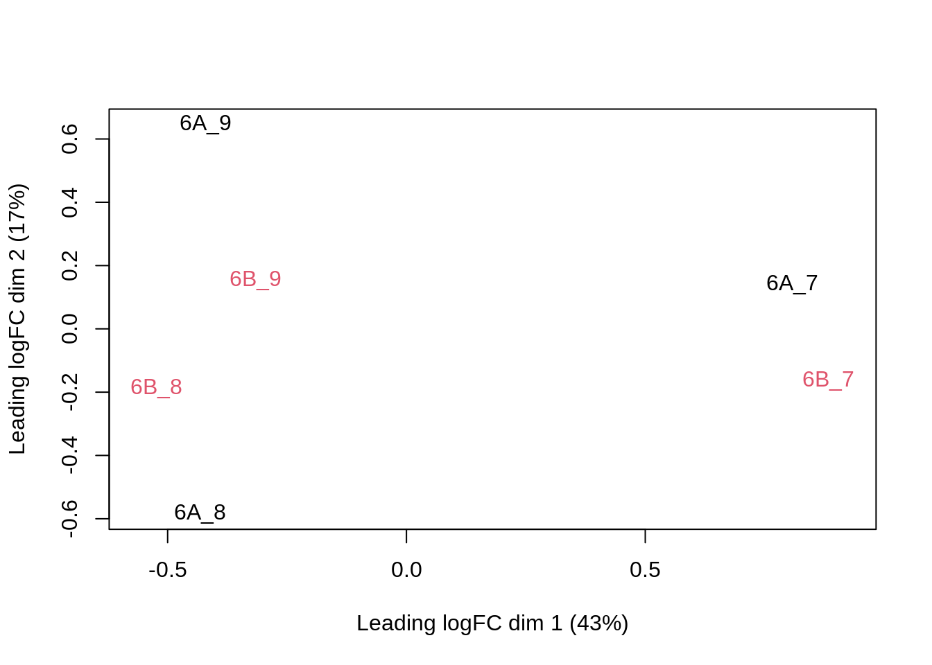

The first axis in the plot is showing the leading log fold changes (differences on the log scale) between the samples. We notice that the leading differences in the peptide data seems to be driven by technical variability. Indeed, the samples do not seem to be clearly separated according to the spike-in condition.

4.5 Protein aggregation

• Here, we use median summarization in aggregateFeatures.
• Note, that this is a suboptimal normalisation procedure!
• By default robust summarization is recommend MsCoreUtils::robustSummary, which is suggested as exercise below.

qf <- aggregateFeatures(qf,
  i = "peptideNorm",
  fcol = "Proteins",
  na.rm = TRUE,
  name = "proteinMedian",
  fun = matrixStats::colMedians)

## Your quantitative and row data contain missing values. Please read the
## relevant section(s) in the aggregateFeatures manual page regarding the
## effects of missing values on data aggregation.

qf

## An instance of class QFeatures containing 4 assays:
##  [1] peptideRaw: SummarizedExperiment with 7011 rows and 6 columns 
##  [2] peptideLog: SummarizedExperiment with 7011 rows and 6 columns 
##  [3] peptideNorm: SummarizedExperiment with 7011 rows and 6 columns 
##  [4] proteinMedian: SummarizedExperiment with 1389 rows and 6 columns

assay(qf[["proteinMedian"]]) %>%
  limma::plotMDS(col = as.numeric(qf$condition))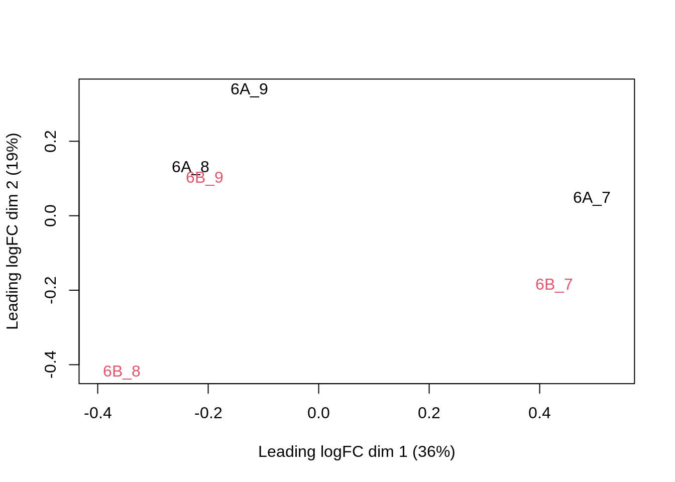

5 Data Analysis

5.1 Estimation

We model the protein level expression values using msqrob. By default msqrob2 estimates the model parameters using robust regression.

We will model the data with a different group mean. The group is incoded in the variable condition of the colData. We can specify this model by using a formula with the factor condition as its predictor: formula = ~condition.

Note, that a formula always starts with a symbol ‘~’.

qf <- msqrob(object = qf,
             i = "proteinMedian",
             formula = ~condition,
             overwrite = TRUE)

rowData(qf[["proteinMedian"]])[, c("Proteins", ".n", "msqrobModels")]

## DataFrame with 1389 rows and 3 columns
##                                Proteins        .n       msqrobModels
##                             <character> <integer>             <list>
## O00762ups|UBE2C_HUMAN_UPS O00762ups|...         2      StatModel:rlm
## P00167ups|CYB5_HUMAN_UPS  P00167ups|...         1 StatModel:fitError
## P00441ups|SODC_HUMAN_UPS  P00441ups|...         3      StatModel:rlm
## P00709ups|LALBA_HUMAN_UPS P00709ups|...         3      StatModel:rlm
## P00915ups|CAH1_HUMAN_UPS  P00915ups|...         1 StatModel:fitError
## ...                                 ...       ...                ...
## sp|Q99258|RIB3_YEAST      sp|Q99258|...         4      StatModel:rlm
## sp|Q99260|YPT6_YEAST      sp|Q99260|...         1 StatModel:fitError
## sp|Q99287|SEY1_YEAST      sp|Q99287|...         1      StatModel:rlm
## sp|Q99383|HRP1_YEAST      sp|Q99383|...         3      StatModel:rlm
## sp|Q99385|VCX1_YEAST      sp|Q99385|...         1 StatModel:fitError

5.2 Inference

First, we extract the parameter names of the model by looking at the first model. The models are stored in the row data of the assay under the default name msqrobModels.

getCoef(rowData(qf[["proteinMedian"]])$msqrobModels[[1]])

## (Intercept)  conditionB 
##   -2.793005    1.541958

We can also explore the design of the model that we specified using the the package ExploreModelMatrix

library(ExploreModelMatrix)
VisualizeDesign(colData(qf),~condition)$plotlist[[1]]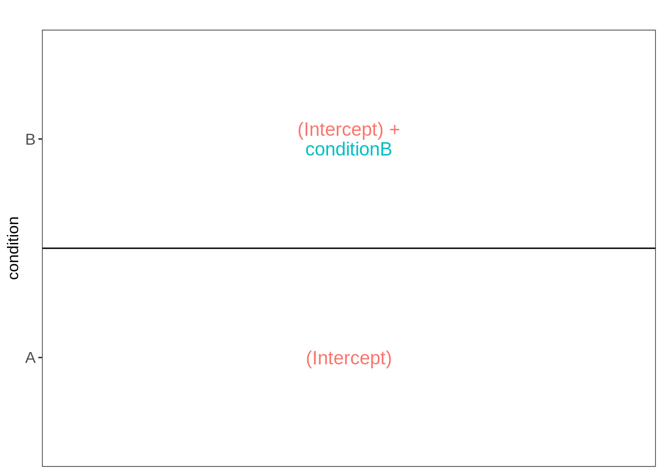

Spike-in condition A is the reference class. So the mean log2 expression for samples from condition A is ‘(Intercept). The mean log2 expression for samples from condition B is’(Intercept)+conditionB’.

Hence, the average log2 fold change between condition b and condition a is modelled using the parameter ‘conditionB’. Thus, we assess the contrast ‘conditionB = 0’ with our statistical test.

L <- makeContrast("conditionB=0", parameterNames = c("conditionB"))
qf <- hypothesisTest(object = qf, i = "proteinMedian", contrast = L)

5.3 Volcano plot

tmp <- rowData(qf[["proteinMedian"]])$conditionB[complete.cases(rowData(qf[["proteinMedian"]])$conditionB),]
tmp$shapes <- 16

volcanoMedian<- ggplot(tmp,
                  aes(x = logFC, y = -log10(pval), color = adjPval < 0.05)) +
    geom_point(cex = 2.5, shape = tmp$shapes) +
    scale_color_manual(values = alpha(c("black", "red"), 0.5)) +
    theme_bw() +
    ggtitle(paste0("Median: TP = ",
                   sum(tmp$adjPval<0.05&grepl(rownames(tmp), pattern = "UPS"), na.rm = TRUE),
                   " FP = ",
                   sum(tmp$adjPval<0.05&!grepl(rownames(tmp), pattern ="UPS"), na.rm = TRUE)))
volcanoMedian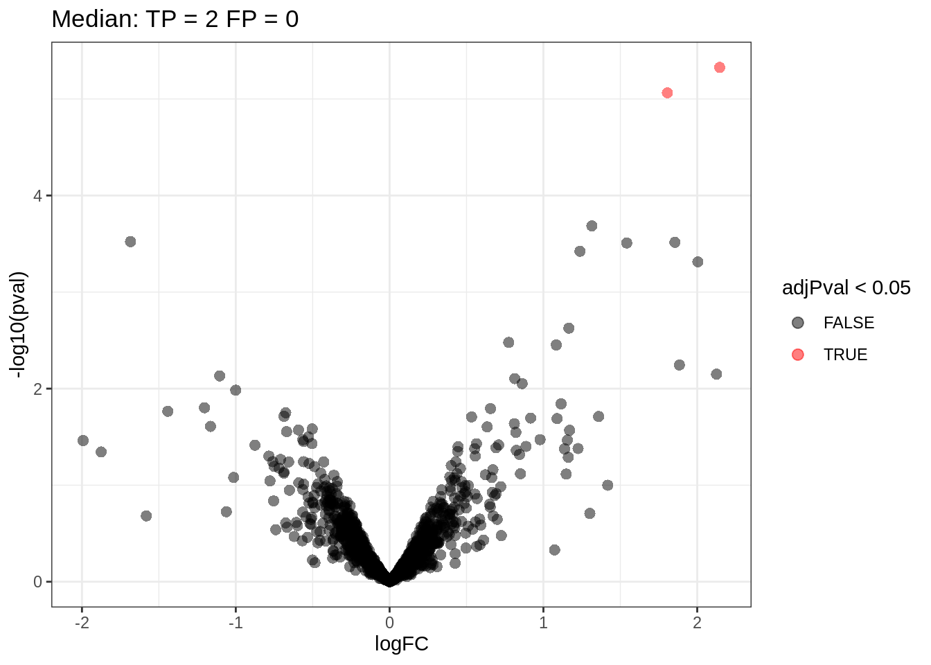

Note, that only 2 proteins are found to be differentially abundant.

5.4 Heatmap

We first select the names of the proteins that were declared significant

sigNames <- rowData(qf[["proteinMedian"]])$conditionB %>%
  rownames_to_column("proteinMedian") %>%
  filter(adjPval < 0.05) %>%
  pull(proteinMedian)

heatmap(assay(qf[["proteinMedian"]][sigNames, ]), cexRow = 1, cexCol = 1)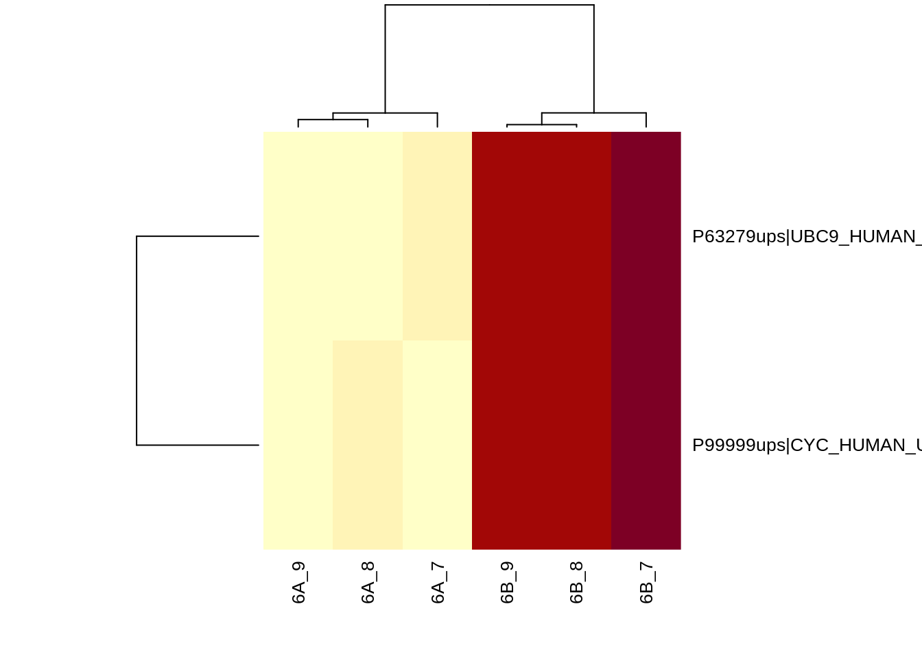

sigProteins <- rowData(qf[["proteinMedian"]])$conditionB %>%
  rownames_to_column("proteinMedian") %>%
   filter(grepl("UPS", proteinMedian)) %>%
  pull(proteinMedian)

heatmap(assay(qf[["proteinMedian"]])[sigProteins, ], cexCol = 1)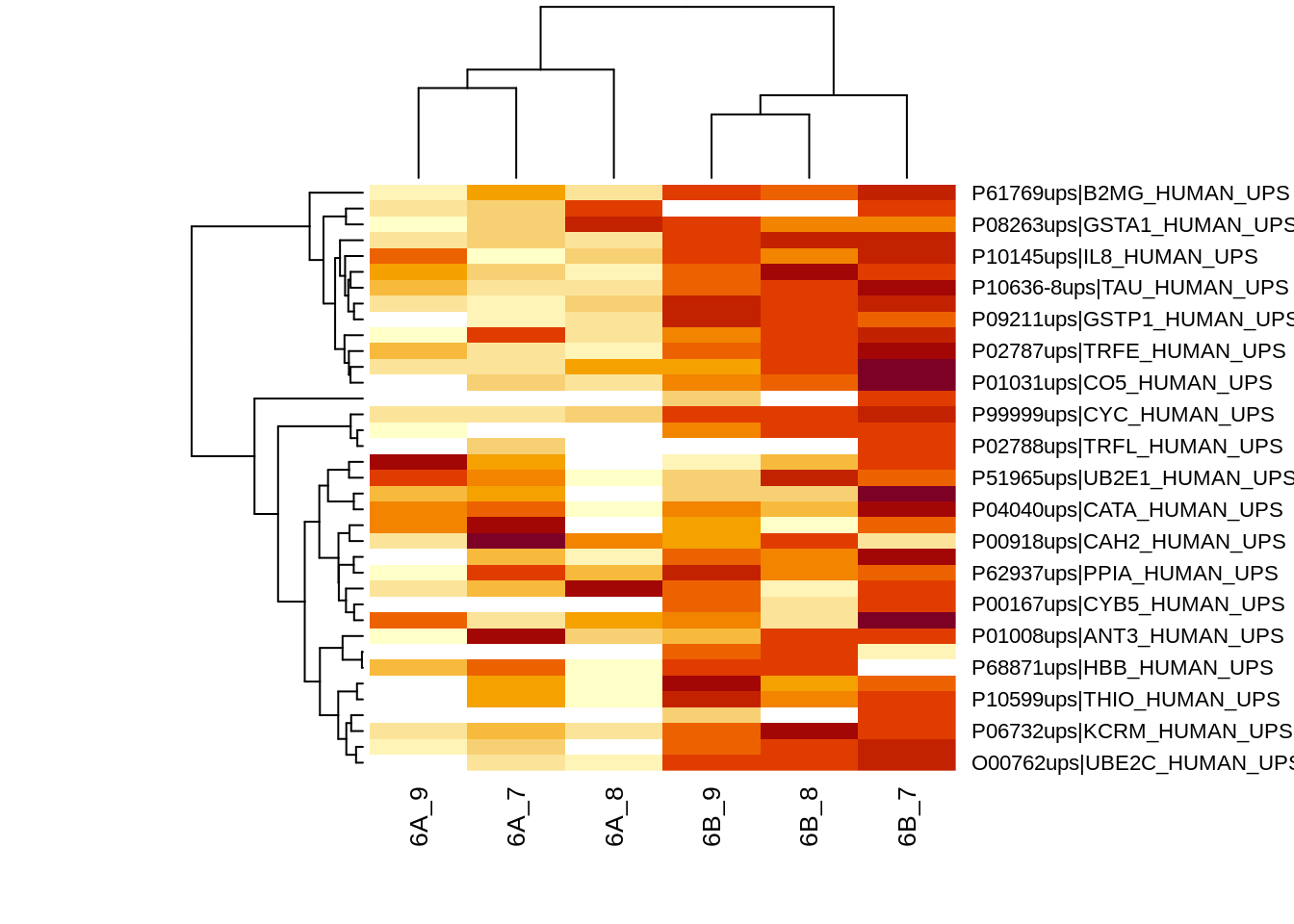

The majority of the proteins are indeed UPS proteins. 1 yeast protein is returned. Note, that the yeast protein indeed shows evidence for differential abundance.

5.5 Boxplots

We create a boxplot of the log2 FC and group according to the whether a protein is spiked or not.

rowData(qf[["proteinMedian"]])$conditionB %>%
  rownames_to_column(var = "protein") %>%
  mutate(ups = grepl("UPS",protein)) %>%
  ggplot(aes(x = ups, y = logFC, fill = ups)) +
  geom_boxplot() +
  theme_bw() +
  geom_hline(yintercept = log2(0.74 / .25), color = "#00BFC4") +
    geom_hline(yintercept = 0, color = "#F8766D")

## Warning: Removed 166 rows containing non-finite values (stat_boxplot).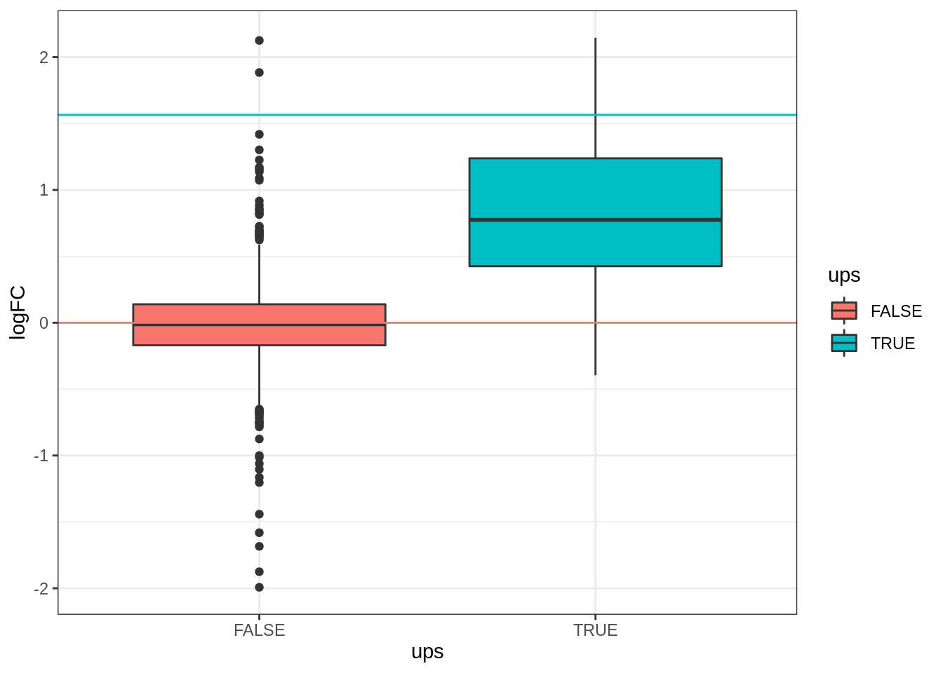

6 Exercise

Repeat the analysis above, aggregating the peptides into proteins using a robust summarisation.

• Note that it isn’t necessary to repeat the whole pipeline. Simply add a new assay, proteinRobust, created from peptideNorm.
• Then rerun the msqrob() estimation and inference using that new assay.

## aggregation
qf <- aggregateFeatures(qf,
  i = "peptideNorm",
  fcol = "Proteins",
  na.rm = TRUE,
  name = "proteinRobust",
  fun = MsCoreUtils::robustSummary)

## Your quantitative and row data contain missing values. Please read the
## relevant section(s) in the aggregateFeatures manual page regarding the
## effects of missing values on data aggregation.

## estimation
qf <- msqrob(object = qf,
             i = "proteinRobust",
             formula = ~ condition,
             overwrite = TRUE)

## inference
L <- makeContrast("conditionB=0", parameterNames = c("conditionB"))
qf <- hypothesisTest(object = qf, i = "proteinRobust", contrast = L)

## volcano plot
tmp <- rowData(qf[["proteinRobust"]])$conditionB[complete.cases(rowData(qf[["proteinRobust"]])$conditionB),]
tmp$shapes <- 16

volcanoRobust <- ggplot(tmp,
                  aes(x = logFC, y = -log10(pval), color = adjPval < 0.05)) +
  geom_point(cex = 2.5, shape = tmp$shapes) +
  scale_color_manual(values = alpha(c("black", "red"), 0.5)) +
  ggtitle(paste0("Median: TP = ",
                 sum(tmp$adjPval<0.05 & grepl(rownames(tmp), pattern ="UPS"), na.rm=TRUE),
                 " FP = ",
                 sum(tmp$adjPval<0.05 & !grepl(rownames(tmp), pattern ="UPS"), na.rm=TRUE)))
volcanoRobust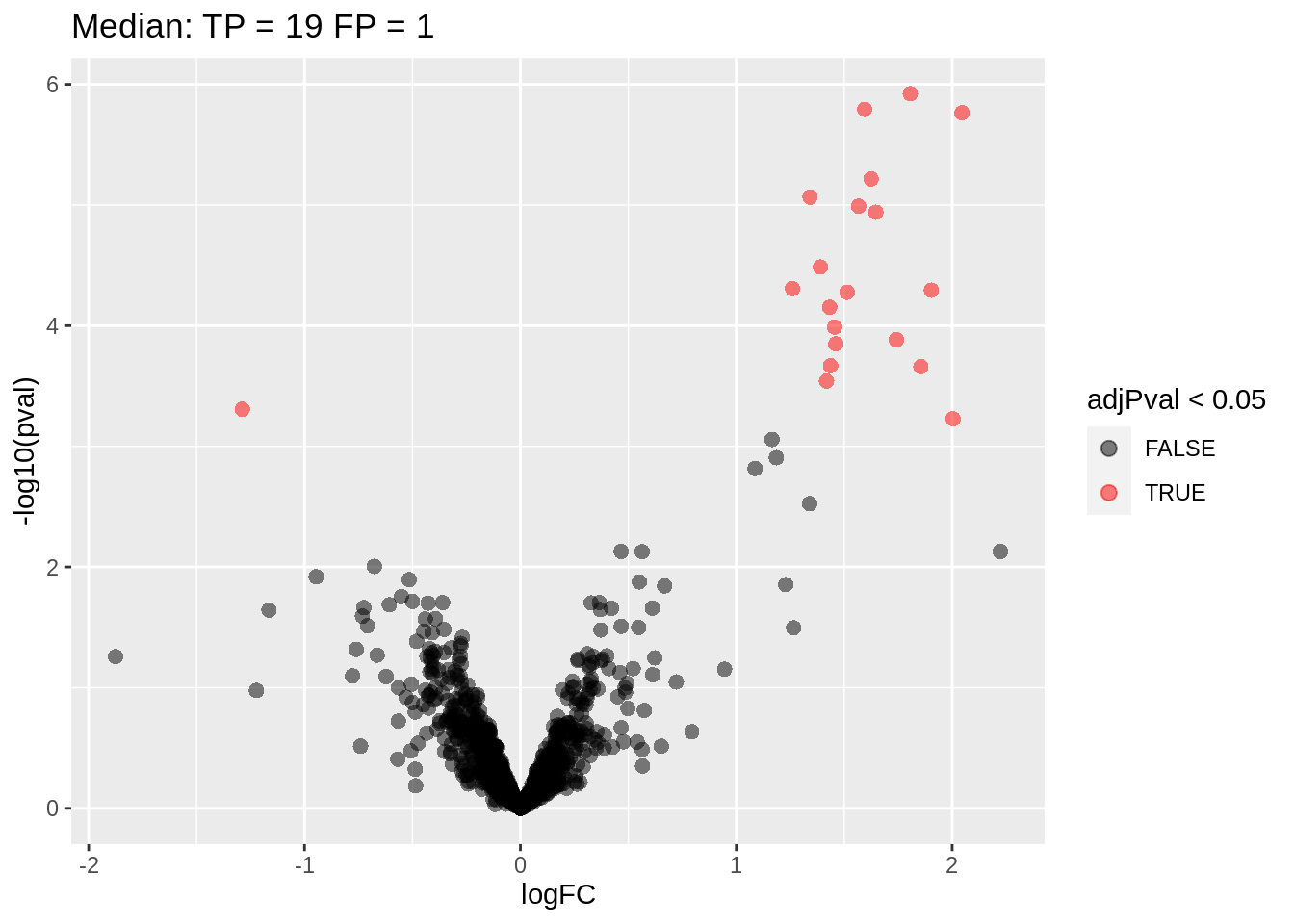

7 Session information

With respect to reproducibility, it is highly recommended to include a session info in your script so that readers of your output can see your particular setup of R.

sessionInfo()

## R version 4.2.1 (2022-06-23)
## Platform: x86_64-pc-linux-gnu (64-bit)
## Running under: Ubuntu 20.04.5 LTS
## 
## Matrix products: default
## BLAS:   /usr/lib/x86_64-linux-gnu/blas/libblas.so.3.9.0
## LAPACK: /usr/lib/x86_64-linux-gnu/lapack/liblapack.so.3.9.0
## 
## locale:
##  [1] LC_CTYPE=C.UTF-8       LC_NUMERIC=C           LC_TIME=C.UTF-8       
##  [4] LC_COLLATE=C.UTF-8     LC_MONETARY=C.UTF-8    LC_MESSAGES=C.UTF-8   
##  [7] LC_PAPER=C.UTF-8       LC_NAME=C              LC_ADDRESS=C          
## [10] LC_TELEPHONE=C         LC_MEASUREMENT=C.UTF-8 LC_IDENTIFICATION=C   
## 
## attached base packages:
## [1] stats4    stats     graphics  grDevices datasets  utils     methods  
## [8] base     
## 
## other attached packages:
##  [1] ExploreModelMatrix_1.8.0    msqrob2_1.4.0              
##  [3] QFeatures_1.6.0             MultiAssayExperiment_1.22.0
##  [5] SummarizedExperiment_1.26.1 Biobase_2.56.0             
##  [7] GenomicRanges_1.48.0        GenomeInfoDb_1.32.4        
##  [9] IRanges_2.30.1              S4Vectors_0.34.0           
## [11] BiocGenerics_0.42.0         MatrixGenerics_1.8.1       
## [13] matrixStats_0.62.0          limma_3.52.3               
## [15] forcats_0.5.2               stringr_1.4.1              
## [17] dplyr_1.0.10                purrr_0.3.4                
## [19] readr_2.1.2                 tidyr_1.2.1                
## [21] tibble_3.1.8                ggplot2_3.3.6              
## [23] tidyverse_1.3.2            
## 
## loaded via a namespace (and not attached):
##   [1] googledrive_2.0.0       minqa_1.2.4             colorspace_2.0-3       
##   [4] ellipsis_0.3.2          XVector_0.36.0          fs_1.5.2               
##   [7] clue_0.3-61             farver_2.1.1            DT_0.25                
##  [10] fansi_1.0.3             lubridate_1.8.0         xml2_1.3.3             
##  [13] codetools_0.2-18        splines_4.2.1           cachem_1.0.6           
##  [16] knitr_1.40              jsonlite_1.8.0          nloptr_2.0.3           
##  [19] broom_1.0.1             cluster_2.1.4           dbplyr_2.2.1           
##  [22] shinydashboard_0.7.2    shiny_1.7.2             BiocManager_1.30.18    
##  [25] compiler_4.2.1          httr_1.4.4              backports_1.4.1        
##  [28] assertthat_0.2.1        Matrix_1.5-1            fastmap_1.1.0          
##  [31] lazyeval_0.2.2          gargle_1.2.1            cli_3.4.0              
##  [34] later_1.3.0             htmltools_0.5.3         tools_4.2.1            
##  [37] igraph_1.3.4            gtable_0.3.1            glue_1.6.2             
##  [40] GenomeInfoDbData_1.2.8  Rcpp_1.0.9              cellranger_1.1.0       
##  [43] jquerylib_0.1.4         vctrs_0.4.1             nlme_3.1-159           
##  [46] rintrojs_0.3.2          xfun_0.33               lme4_1.1-30            
##  [49] rvest_1.0.3             mime_0.12               lifecycle_1.0.2        
##  [52] renv_0.15.5             googlesheets4_1.0.1     zlibbioc_1.42.0        
##  [55] MASS_7.3-58.1           scales_1.2.1            promises_1.2.0.1       
##  [58] hms_1.1.2               ProtGenerics_1.28.0     parallel_4.2.1         
##  [61] AnnotationFilter_1.20.0 yaml_2.3.5              sass_0.4.2             
##  [64] stringi_1.7.8           highr_0.9               boot_1.3-28            
##  [67] BiocParallel_1.30.3     rlang_1.0.5             pkgconfig_2.0.3        
##  [70] bitops_1.0-7            evaluate_0.16           lattice_0.20-45        
##  [73] htmlwidgets_1.5.4       labeling_0.4.2          cowplot_1.1.1          
##  [76] tidyselect_1.1.2        magrittr_2.0.3          R6_2.5.1               
##  [79] generics_0.1.3          DelayedArray_0.22.0     DBI_1.1.3              
##  [82] pillar_1.8.1            haven_2.5.1             withr_2.5.0            
##  [85] MsCoreUtils_1.8.0       RCurl_1.98-1.8          msdata_0.36.0          
##  [88] modelr_0.1.9            crayon_1.5.1            utf8_1.2.2             
##  [91] tzdb_0.3.0              rmarkdown_2.16          grid_4.2.1             
##  [94] readxl_1.4.1            reprex_2.0.2            digest_0.6.29          
##  [97] xtable_1.8-4            httpuv_1.6.6            munsell_0.5.0          
## [100] bslib_0.4.0             shinyjs_2.1.0

---

This work is licensed under the CC BY-SA-4.0 licence.