4. Sparse Singular Value Decomposition

1 Introduction

In high dimensional data the PCs may have unclear interpretation because they depend on all \(p\) original variables.

1.1 Example: Toxicogenomics in early drug development

1.1.1 Background

• Effect of compound on gene expression.

• Insight in action and toxicity of drug in early phase

• Determine activity with bio-assay: e.g. binding afinity of compound to cellwall recepter (target, IC50).

• Early phase: 20 to 50 compounds

• Based on in vitro results one aims to get insight in how to build better compound (higher on-target activity less toxicity.

• Small variantions in moelculair structure lead to variations in BA and gene expression.

• Aim: Build model to predict bio-activity based on gene expression in liver cell line.

1.1.2 Data

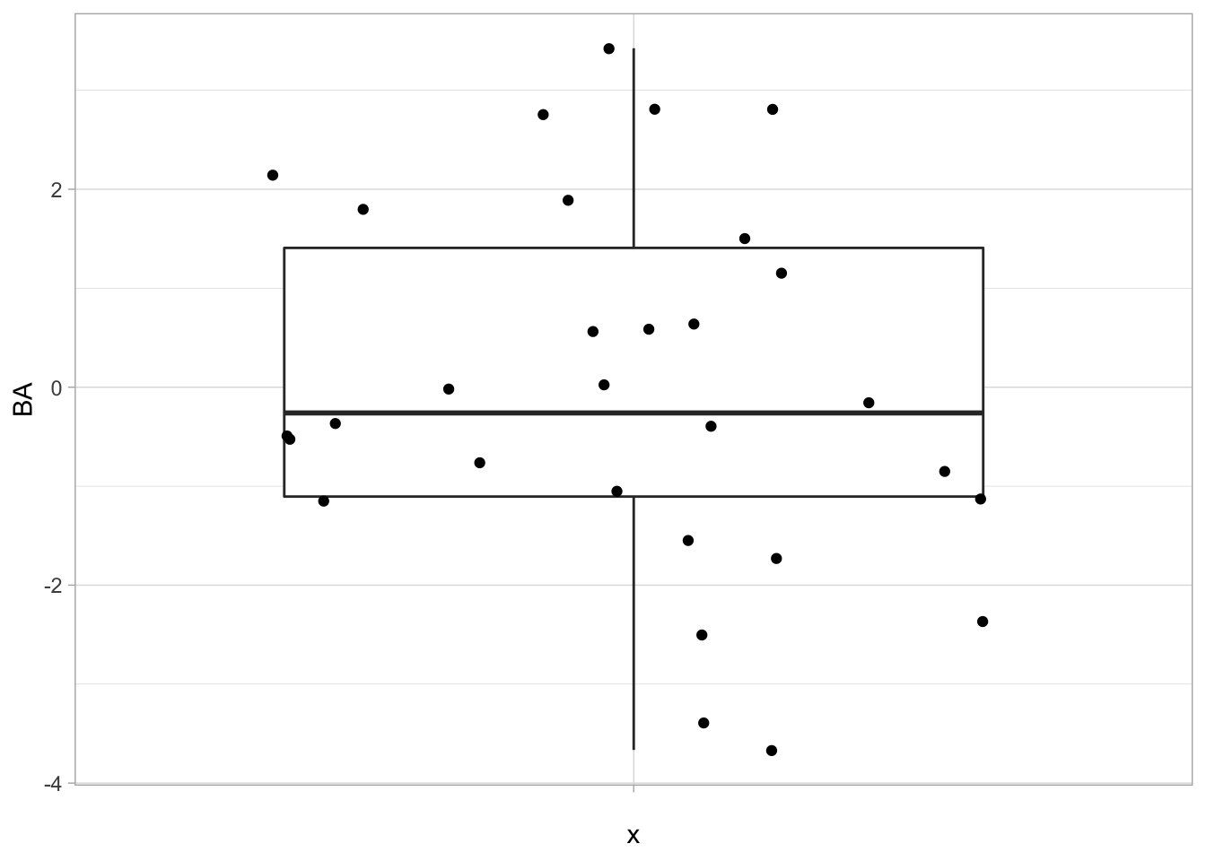
• 30 chemical compounds have been screened for toxicity

• Bioassay data on toxicity screening

• Gene expressions in a liver cell line are profiled for each compound (4000 genes)

toxData <- read_csv(
  "https://raw.githubusercontent.com/statOmics/HDA2020/data/toxDataCentered.csv",
  col_types = cols()
)
svdX <- svd(toxData[,-1])

Data is already centered:

toxData %>%
  colMeans %>%
  range

## [1] -1.434038e-17  2.567391e-17

 toxData %>%
  names %>%
  head

## [1] "BA" "X1" "X2" "X3" "X4" "X5"

• First column contains data on Bioassay.
• The higher the score on Bioassay the more toxic the compound
• Other columns contain data on gene expression X1, … , X4000

1.1.3 Data exploration

toxData %>%
  ggplot(aes(x="",y=BA)) +
  geom_boxplot(outlier.shape=NA) +
  geom_point(position="jitter")

svdX <- toxData[,-1] %>%
  svd

k <- 2
Vk <- svdX$v[,1:k]
Uk <- svdX$u[,1:k]
Dk <- diag(svdX$d[1:k])
Zk <- Uk%*%Dk
colnames(Zk) <- paste0("Z",1:k)
colnames(Vk) <- paste0("V",1:k)

pca <- Zk %>%
  as.data.frame %>%
  mutate(BA = toxData %>% pull(BA)) %>%
  ggplot(aes(x= Z1, y = Z2, color = BA)) +
  geom_point(size = 3) +
  scale_colour_gradient2(low = "blue",mid="white",high="red") +
  geom_point(size = 3, pch = 21, color = "black")
pca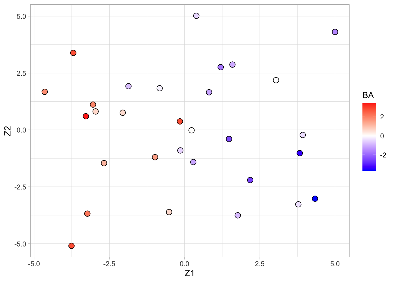

• Scores on the first two principal components (or MDS plot). - Each point corresponds to a compound.
• Color code refers to the toxicity score (higher score more toxic).
• Clear separation between compounds according to toxicity.

---

• Next logic step in a PCA is to interpret the principal components.
• We thus have to assess the loadings.
• We can add a vector for each gene to get a biplot, but this would require plotting 4000 vectors, which would render the plot unreadable.

Alternative graph to look at the many loadings of the first two PCs.

grid.arrange(
  Vk %>%
    as.data.frame %>%
    mutate(geneID = 1:nrow(Vk)) %>%
    ggplot(aes(x = geneID, y = V1)) +
    geom_point(pch=21) +
    geom_hline(yintercept = c(-2,0,2)*sd(Vk[,1]), col = "red") ,
  Vk %>%
    as.data.frame %>%
    mutate(geneID = 1:nrow(Vk)) %>%
    ggplot(aes(x = geneID, y = V2)) +
    geom_point(pch=21) +
    geom_hline(yintercept = c(-2,0,2)*sd(Vk[,2]), col = "red"),
  ncol=2)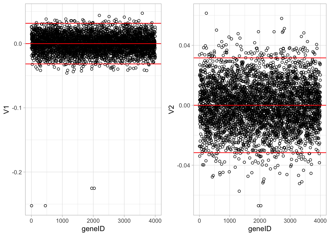

• It is almost impossible to interpret the PCs because there are 4000 genes contributing to each PC.

• In an attempt to find the most important genes (in the sense that they drive the interpretation of the PCs), the plots show horizontal reference lines: the average of the loadings, and the average ± twice the standard deviation of the loadings. In between the lines we expects about 95% of the loadings (if they were normally distributed).

• The points outside the band come from the genes that have rather large loadings (in absolute value) and hence are important for the interpretation of the PCs.

• Note, that particularly for the first PC, only a few genes show a markedly large loadings that are negative. This means that an upregulation of these genes will lead to low scores on PC1.

• These genes will very likely play an important role in the toxicity mechanism.

• Indeed, low scores on PC1 are in the direction of more toxicity.

---

1.2 Sparse matrix decomposition

Basic idea of sparse matrix decomposition of an \(n \times p\) matrix \(\mathbf{X}\)}

Find a rank \(k\) approximation of \(\mathbf{X}\) of the form \[ \mathbf{X}_k = \sum_{j=1}^k \delta_j \mathbf{u}_j\mathbf{v}_j^t \] such that many of the elements in the \(\mathbf{v}_j\) and or \(\mathbf{u}_j\) are exactly zero.

We focus on the Penalised Matrix Decomposition (PMD) method of Witten et al. (2009, Biostatistics, 10, 3, 515-534).

When many of the loadings in \(\mathbf{v}_j\) are zero, the interpretation of the PC only depends on the features that correspond to the remaining non-zero loadings.

---

2 Penalised Matrix Decomposition

2.1 Rank 1 approximation

The rank-1 PMD approximation of the \(n \times p\) matrix \(\mathbf{X}\) is of the form \[ \mathbf{X}_1 = \delta_1\mathbf{u}_1\mathbf{v}_1^t, \]

and it is the solution to the following minimisation problem: \[ \min_{\delta,u,v} \Vert \mathbf{X} - \delta\mathbf{u}\mathbf{v}^t\Vert_F^2 \text{ subject to } \delta \geq 0, \Vert \mathbf{u}\Vert_2^2=\Vert \mathbf{v}\Vert_2^2=1, \Vert\mathbf{u}\Vert_1\leq c_1, \Vert \mathbf{v}\Vert_1 \leq c_2 \]

for some user-defined constants \(c_1,c_2>0\).

The constraints \(\Vert\mathbf{u}\Vert_1\leq c_1\) and \(\Vert \mathbf{v}\Vert_1 \leq c_2\) are known as \(L_1\) or lasso constraints.

Note, \[ \Vert\mathbf{u}\Vert_1\ = \sum_{i=1}^n \vert u_i \vert \text{ and }\Vert\mathbf{v}\Vert_1\ = \sum_{i=1}^p \vert v_i\vert. \]

If \(c_1=+\infty\), then the constraint on \(\mathbf{u}\) is removed (similar for \(c_2\)).

---

Note that \[ \min_{\delta,u,v} \Vert \mathbf{X} - \delta\mathbf{u}\mathbf{v}^t\Vert_F^2 = \min_{A:\text{rank}(A)=1} \Vert \mathbf{X} - A\Vert_F^2 \] with \(A=X_1\) (truncated SVD of \(\mathbf{X}\), truncated after 1 term). However, the PMD requires a constrained minimisation. The unconstrained solution arises with \(c_1=c_2=+\infty\).

Note that \(\Vert \mathbf{u}\Vert_2^2=\Vert \mathbf{v}\Vert_2^2=1\) may also be written as \(\mathbf{u}^t\mathbf{u}=\mathbf{v}^t\mathbf{v}=1\) (i.e. the vectors are normalised, just like for the singular vectors of the SVD).

• We also applied the \(L_1\) constraint to the least-squares estimator of the regression parameters in a linear regression model.

• Effect was that many of the parameter estimates are set exactly to zero.

• Here, the same effect will take place. Many of the elements in \(\mathbf{u}\) and \(\mathbf{v}\) will be set exactly to zero.

• In particular, the smaller \(c_2\), the more elements of \(\mathbf{v}\) will be set to zero (shrinkage).

• Similarly, the smaller \(c_1\), the more elements of \(\mathbf{u}\) will be set to zero.

• The choice of \(c_1\) and \(c_2\) depends on the objective of the data analysis and will be discussed later.

The solution is known as a rank-1 PMD approximation of \(\mathbf{X}\) because \(\delta_1\mathbf{u}_1\mathbf{v}_1^t\) is a matrix of rank 1.

---

2.2 Rank-2 approximation

The rank-2 PMD approximation is found as follows:

1. find the rank-1 PMD as before: \(\mathbf{X}_1=\delta_1\mathbf{u}_1\mathbf{v}_1^t\);

2. compute \[ \tilde{\mathbf{X}}_2 = \mathbf{X}-\mathbf{X}_1, \]

and compute the rank-1 PMD of \(\tilde{\mathbf{X}}_2\), which gives \(\delta_2, \mathbf{u}_2, \mathbf{v}_2\);

3. the rank-2 PMD of \(\mathbf{X}\) is then given by \[ \mathbf{X}_2 = \delta_1\mathbf{u}_1\mathbf{v}_1^t+\delta_2\mathbf{u}_2\mathbf{v}_2^t. \]

Note that the \(\mathbf{u}\)’s and \(\mathbf{v}\)’s are not necessarily orthogonal (only if \(c_1, c_2=+\infty\)).

---

2.3 Rank-k approximation

The rank-\(k\) PMD approximation is found as follows:

1. find the rank-1 PMD as before: \(\tilde{\mathbf{X}}_1=\delta_1\mathbf{u}_1\mathbf{v}_1^t\);

2. set \(j=1\);

3. compute \[ \tilde{\mathbf{X}}_{j+1} = \mathbf{X}-\tilde{\mathbf{X}}_1-\cdots - \tilde{\mathbf{X}}_j, \] and compute the rank-1 PMD of \(\tilde{\mathbf{X}}_{j+1}\), which gives \(\delta_{j+1}, \mathbf{u}_{j+1}, \mathbf{v}_{j+1}\);

4. if \(j<k\), increase \(j\) with one and go back to step 3; otherwise go to step 5;

5. the rank-\(k\) PMD of \(\mathbf{X}\) is then given by \[ \mathbf{X}_k = \sum_{j=1}^k \delta_j\mathbf{u}_j\mathbf{v}_j^t. \]

Without the \(L_1\) constraints, this algorithm gives the ordinary SVD.

As before the \(\delta_j\)s, \(\mathbf{u}_j\)s and \(\mathbf{v}_j\)s are stacked into matrices \(\mathbf{D}_k\), \(\mathbf{U}_k\) and \(\mathbf{V}_k\): \(\mathbf{X}_k = \mathbf{U}_k\mathbf{D}_k\mathbf{V}_k^t\).

Note that the \(\mathbf{u}\) vectors are generally not orthogonal (i.e. \(\mathbf{u}_i^t\mathbf{u}_j\neq 0\) for \(i\neq j\)) (the same holds for the \(\mathbf{v}\) vectors).

---

2.4 Sparse PCA via PMD

Just like the SVD can be used to find the PCA solution, the PMD can be used to find a sparse PCA solution (SPC).

For a PCA, it is only important to have sparse loadings (in the \(\mathbf{v}\)s); the scores (involving the \(\mathbf{u}\)s) need not be sparse.

The rank-1 solutions thus satisfy \[ \min_{\delta,u,v} \Vert \mathbf{X} - \delta\mathbf{u}\mathbf{v}^t\Vert_F^2 \text{ subject to } \delta \geq 0, \Vert \mathbf{u}\Vert_2^2=\Vert \mathbf{v}\Vert_2^2=1, \Vert \mathbf{v}\Vert_1 \leq c \] (i.e. no sparsity constraint on \(\mathbf{u}\)).

Hence the PCA scores \[ \mathbf{Z}_k = \mathbf{U}_k\mathbf{D}_k \] relate to \(\mathbf{X}_k\) through the sparse loadings in \(\mathbf{V}_k\).

---

It can be shown that the SPC solution (rank-1) also maximises \[ \mathbf{v}^t\mathbf{X}^t\mathbf{X}\mathbf{v} \text{ subject to } \Vert \mathbf{u}\Vert_2^2=\Vert \mathbf{v}\Vert_2^2=1, \Vert \mathbf{v}\Vert_1 \leq c \] (i.e. it maximises the variance of the PCs, subject to sparsity constraint on loadings).

From these two slides we may conclude that we can use the PMD as the basis of a sparse PCA, and that the interpretation is as before in terms of maximising variance. Only now we hope that only a few features will give a non-zero loading in the \(\mathbf{v}\)-vectors. Biplots may again be constructed (with fewer vectors to be plotted).

---

3 Toxicogenomics analysis with a sparse PCA

3.1 SPCA

library(PMA)

spcX <- SPC(
  toxData[,-1] %>%
    as.matrix,
  K=30,
  sumabsv = 5)

## 12345678910111213141516171819
## 1234567891011121314151617181920
## 1234567891011121314151617181920
## 1234567891011121314151617181920
## 1234567891011121314151617181920
## 1234567891011121314151617181920
## 1234567891011121314151617181920
## 1234567891011121314151617181920
## 1234567891011121314151617181920
## 1234567891011121314151617181920
## 1234567891011121314151617181920
## 1234567891011121314151617181920
## 1234567891011121314151617181920
## 1234567891011121314151617181920
## 1234567891011121314151617181920
## 1234567891011121314151617181920
## 1234567891011121314151617181920
## 1234567891011121314151617181920
## 1234567891011121314151617181920
## 1234567891011121314151617181920
## 1234567891011121314151617181920
## 1234567891011121314151617181920
## 1234567891011121314151617181920
## 1234567891011121314151617181920
## 1234567891011121314151617181920
## 1234567891011121314151617181920
## 1234567891011121314151617181920
## 1234567891011121314151617181920
## 1234567891011121314151617181920
## 1234567891011121314151617181920

par(mfrow=c(1,2))
barplot(spcX$d^2,ylab="eigenvalue",cex.lab=1.5)
barplot(spcX$prop.var.explained,
     ylab="cummulative variance",cex.lab=1.5)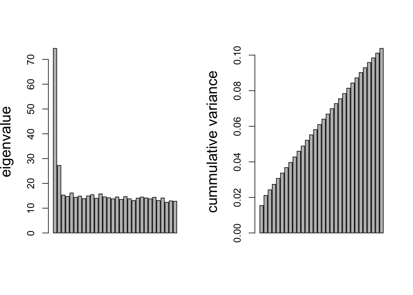

• The plot on the left shows the eigenvalues (squared singular values) from the PMD.

  • This suggests that the first one or two are the most important, but all eigenvalues remain substantially larger than zero.

• The figure on the right shows the cumulative percentage of variance retained in the PCs.

  • These percentages are now no longer calculated as before as ratio’s of sums of eigenvalues.
  • A more complicated calculation is required now, because the PCs are no longer uncorrelated with one another.
  • Thus part of the information (variance) of one PC is shared with part of the information of another PCs (i.e. non-zero correlation or covariance).

3.2 Loading

Loadings of the first two PCs, with constraint \(\Vert\mathbf{v}\Vert_1 < 5\).

k <- 2
Vk <- spcX$v[,1:k]
colnames(Vk) <- paste0("V",1:k)

grid.arrange(
  Vk %>%
    as.data.frame %>%
    mutate(geneID = 1:nrow(Vk)) %>%
    ggplot(aes(x = geneID, y = V1)) +
    geom_point(pch=21) +
    geom_hline(yintercept = c(-2,0,2)*sd(Vk[,1]), col = "red") ,
  Vk %>%
    as.data.frame %>%
    mutate(geneID = 1:nrow(Vk)) %>%
    ggplot(aes(x = geneID, y = V2)) +
    geom_point(pch=21) +
    geom_hline(yintercept = c(-2,0,2)*sd(Vk[,2]), col = "red"),
  ncol=2)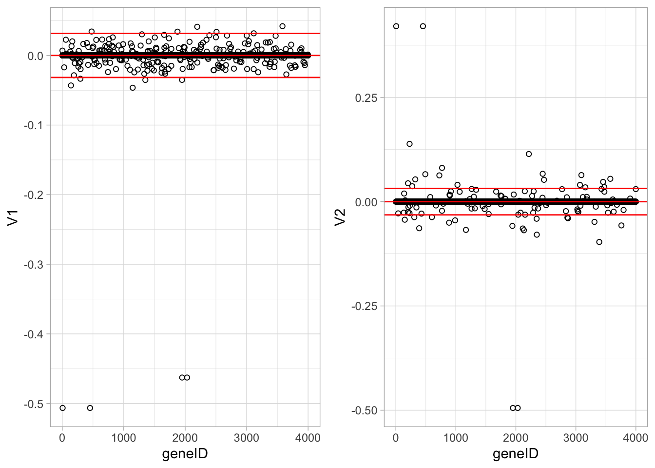

These plots show the loadings of the first two sparse PCs. Many of the loadings are now exactly equal to zero. Only few genes show large loadings.

3.3 Change constraint

We now repeat the analysis, but with the constraint \(\Vert \mathbf{v} \Vert_1 < 1\). This gives a much sparser solution with only two genes with non-zero loadings in each dimension.

spcX1 <- SPC(
  toxData[,-1] %>%
    as.matrix,
  K=30,
  sumabsv = 1)

## 12
## 12
## 12
## 12
## 12
## 12
## 12
## 12
## 12
## 12
## 12
## 12
## 12
## 12
## 12
## 12
## 12
## 12
## 12
## 12
## 12
## 12
## 12
## 12
## 12
## 12
## 12
## 12
## 12
## 12

k <- 2
Vk <- spcX1$v[,1:k]
colnames(Vk) <- paste0("V", 1:k)

grid.arrange(
  Vk %>%
    as.data.frame %>%
    mutate(geneID = 1:nrow(Vk)) %>%
    ggplot(aes(x = geneID, y = V1)) +
    geom_point(pch=21) +
    geom_hline(yintercept = c(-2,0,2)*sd(Vk[,1]), col = "red") ,
  Vk %>%
    as.data.frame %>%
    mutate(geneID = 1:nrow(Vk)) %>%
    ggplot(aes(x = geneID, y = V2)) +
    geom_point(pch=21) +
    geom_hline(yintercept = c(-2,0,2)*sd(Vk[,2]), col = "red"),
  ncol=2)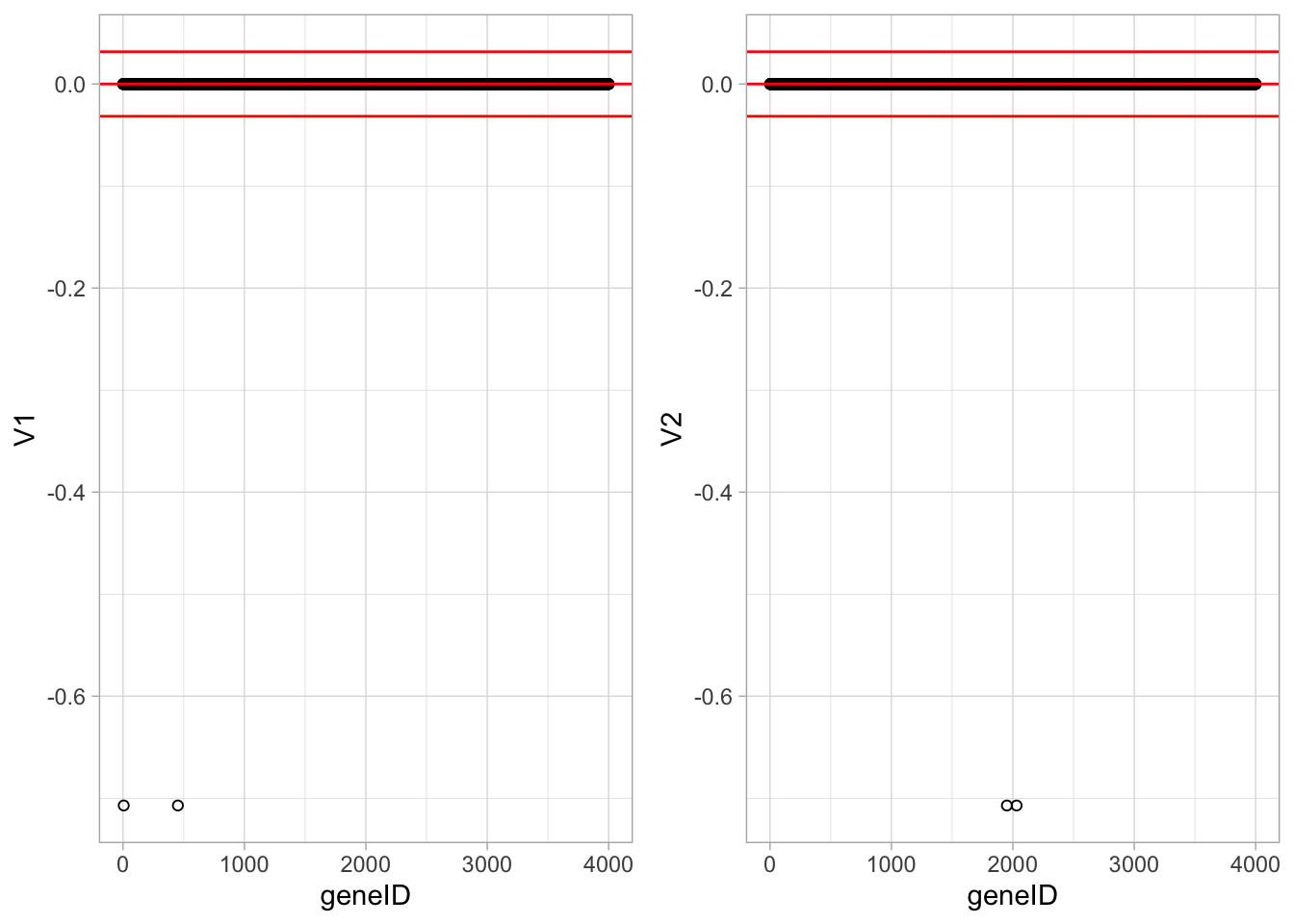

---

We now repeat the analysis, but with the constraint \(\Vert \mathbf{v} \Vert_1 < 10\). This gives a much less sparse solution with several genes with non-zero loadings.

spcX10 <- SPC(
  toxData[,-1] %>%
    as.matrix,
  K=30,
  sumabsv = 10)

## 1234567891011121314151617181920
## 1234567891011121314151617181920
## 1234567891011121314151617181920
## 1234567891011121314151617181920
## 1234567891011121314151617181920
## 1234567891011121314151617181920
## 1234567891011121314151617181920
## 1234567891011121314151617181920
## 1234567891011121314151617181920
## 1234567891011121314151617181920
## 1234567891011121314151617181920
## 1234567891011121314151617181920
## 1234567891011121314151617181920
## 1234567891011121314151617181920
## 1234567891011121314151617181920
## 1234567891011121314151617181920
## 1234567891011121314151617181920
## 1234567891011121314151617181920
## 1234567891011121314151617181920
## 1234567891011121314151617181920
## 1234567891011121314151617181920
## 1234567891011121314151617181920
## 1234567891011121314151617181920
## 1234567891011121314151617181920
## 1234567891011121314151617181920
## 1234567891011121314151617181920
## 1234567891011121314151617181920
## 1234567891011121314151617181920
## 1234567891011121314151617181920
## 1234567891011121314151617181920

k <- 2
Vk <- spcX10$v[,1:k]
colnames(Vk) <- paste0("V",1:k)

grid.arrange(
  Vk %>%
    as.data.frame %>%
    mutate(geneID = 1:nrow(Vk)) %>%
    ggplot(aes(x = geneID, y = V1)) +
    geom_point(pch=21) +
    geom_hline(yintercept = c(-2,0,2)*sd(Vk[,1]), col = "red") ,
  Vk %>%
    as.data.frame %>%
    mutate(geneID = 1:nrow(Vk)) %>%
    ggplot(aes(x = geneID, y = V2)) +
    geom_point(pch=21) +
    geom_hline(yintercept = c(-2,0,2)*sd(Vk[,2]), col = "red"),
  ncol=2)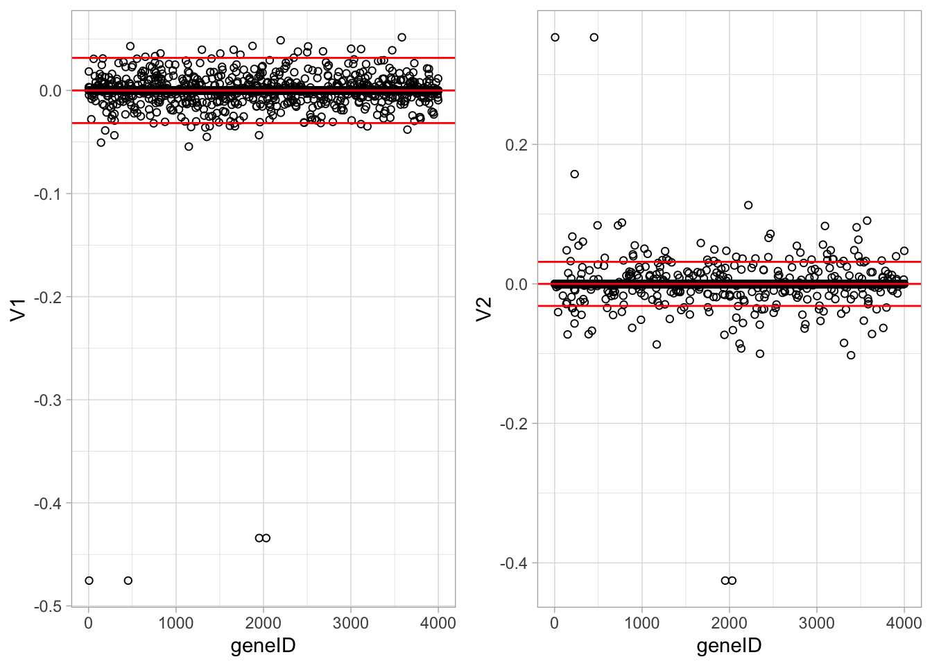

---

3.4 Variance explained

Variance explained for \(c=1,5,10\) and \(+\infty\).

data.frame(
  PCs = 1:30,
  "c1" = spcX1$prop.var.explained,
  "c5" = spcX$prop.var.explained,
  "c10" = spcX10$prop.var.explained,
  "conventional" = cumsum(svdX$d^2)/sum(svdX$d^2)
  ) %>%
  gather("method","varExpl",-1) %>%
  ggplot(aes(x = PCs, y = varExpl, color = method)) +
  geom_line() +
  geom_point() +
  ylab("Variance explained (%)")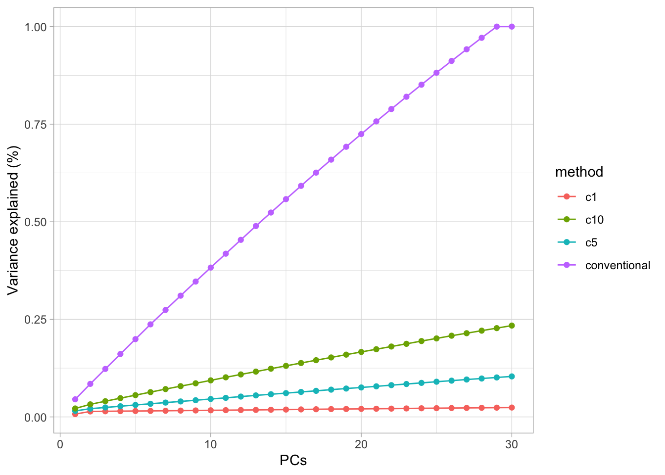

This graph illustrates that the percentages of variance explained by the PCs are smaller for sparser solutions. Thus in choosing an appropriate penalty parameter \(c_2\) one should not only look at the sparseness of the solution, but also at the percentage of variance contained in the first few PCs. If this percentage is very small, then the graphs of the scores (or biplots) are no longer very informative (i.e. they will not tell the full story). Thus a compromise must be looked for.

library(latex2exp)

Uk5 <- spcX$u[,1:k]
Dk5 <- diag(spcX$d[1:k])
Zk5 <- Uk5%*%Dk5
colnames(Zk5) <- paste0("Z",1:k)

spc5 <- Zk5 %>%
  as.data.frame %>%
  mutate(BA = toxData %>% pull(BA)) %>%
  ggplot(aes(x= Z1, y = Z2, color = BA)) +
  geom_point(size = 3) +
  scale_colour_gradient2(low = "blue",mid="white",high="red") +
  geom_point(size = 3, pch = 21, color = "black") +
  ggtitle(TeX("$c_2 = 5$"))

Uk1 <- spcX1$u[,1:k]
Dk1 <- diag(spcX1$d[1:k])
Zk1 <- Uk1%*%Dk1
colnames(Zk1) <- paste0("Z",1:k)

spc1 <- Zk1 %>%
  as.data.frame %>%
  mutate(BA = toxData %>% pull(BA)) %>%
  ggplot(aes(x= Z1, y = Z2, color = BA)) +
  geom_point(size = 3) +
  scale_colour_gradient2(low = "blue",mid="white",high="red") +
  geom_point(size = 3, pch = 21, color = "black") +
  ggtitle(TeX("$c_2 = 1$"))

Uk10 <- spcX10$u[,1:k]
Dk10 <- diag(spcX10$d[1:k])
Zk10 <- Uk10%*%Dk10
colnames(Zk10) <- paste0("Z",1:k)

spc10 <- Zk10 %>%
  as.data.frame %>%
  mutate(BA = toxData %>% pull(BA)) %>%
  ggplot(aes(x= Z1, y = Z2, color = BA)) +
  geom_point(size = 3) +
  scale_colour_gradient2(low = "blue",mid="white",high="red") +
  geom_point(size = 3, pch = 21, color = "black") +
  ggtitle(TeX("$c_2 = 10$"))

grid.arrange(spc1, spc5, spc10, pca + ggtitle(TeX("$c_2 = \\infty")), ncol = 2)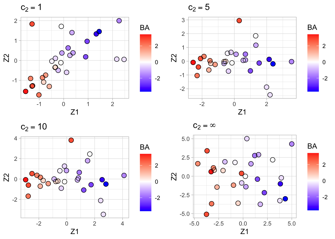

Finally we show the plots of the scores on the first two sparse PCs for \(c_2=1\) (top-left), \(c_2=5\) (top-right) and \(c_2=10\) (bottom-left) and \(c_2=\infty\) (bottom-right, convention SVD).

Note, that the most sparse solution (top-left) shows a strong positive correlation between the first two PCs (as a consequence of the loss of orthogonality of the singular vectors).

All graphs succeed quite well in separating the toxic from the non-toxic compounds based on their gene expression.

• Hence, we may expect that the two genes identified from the most sparse solution play an important role in the development of toxic effects.

• Note, however, that our data analysis did not provide a scientific proof for this conclusion: (sparse) PCA is only an exploratory or descriptive data analysis method that helps the data-analyst to gain insight into the data.

• The fact that we found a few genes that appear to be associated with toxicity is of course a nice result.

• It is important to understand that the toxicity outcome was not used in the (sparse) PCA. We only used the toxicity to color the points in the graphs. PCA is an unsupervised method.

Acknowledgement

• Olivier Thas for sharing his materials of Analysis of High Dimensional Data 2019-2020, which I used as the starting point for this chapter.

Session info

Session info

## [1] "2021-05-11 14:44:38 UTC"

## ─ Session info ───────────────────────────────────────────────────────────────
##  setting  value                       
##  version  R version 4.0.5 (2021-03-31)
##  os       macOS Catalina 10.15.7      
##  system   x86_64, darwin17.0          
##  ui       X11                         
##  language (EN)                        
##  collate  en_US.UTF-8                 
##  ctype    en_US.UTF-8                 
##  tz       UTC                         
##  date     2021-05-11                  
## 
## ─ Packages ───────────────────────────────────────────────────────────────────
##  package                * version    date       lib
##  AIMS                   * 1.22.0     2020-10-27 [1]
##  amap                     0.8-18     2019-12-12 [1]
##  AnnotationDbi            1.52.0     2020-10-27 [1]
##  AnnotationHub          * 2.22.1     2021-04-16 [1]
##  askpass                  1.1        2019-01-13 [1]
##  assertthat               0.2.1      2019-03-21 [1]
##  backports                1.2.1      2020-12-09 [1]
##  beachmat                 2.6.4      2020-12-20 [1]
##  beeswarm                 0.3.1      2021-03-07 [1]
##  Biobase                * 2.50.0     2020-10-27 [1]
##  BiocFileCache          * 1.14.0     2020-10-27 [1]
##  BiocGenerics           * 0.36.1     2021-04-16 [1]
##  BiocManager              1.30.15    2021-05-11 [1]
##  BiocNeighbors            1.8.2      2020-12-07 [1]
##  BiocParallel             1.24.1     2020-11-06 [1]
##  BiocSingular             1.6.0      2020-10-27 [1]
##  BiocVersion              3.12.0     2020-05-14 [1]
##  biomaRt                * 2.46.3     2021-02-11 [1]
##  bit                      4.0.4      2020-08-04 [1]
##  bit64                    4.0.5      2020-08-30 [1]
##  bitops                   1.0-7      2021-04-24 [1]
##  blob                     1.2.1      2020-01-20 [1]
##  boot                   * 1.3-28     2021-05-03 [1]
##  bootstrap                2019.6     2019-06-17 [1]
##  breastCancerMAINZ      * 1.28.0     2020-10-29 [1]
##  broom                    0.7.6      2021-04-05 [1]
##  bslib                    0.2.4      2021-01-25 [1]
##  cachem                   1.0.4      2021-02-13 [1]
##  callr                    3.7.0      2021-04-20 [1]
##  CCA                    * 1.2.1      2021-03-01 [1]
##  cellranger               1.1.0      2016-07-27 [1]
##  class                    7.3-18     2021-01-24 [2]
##  cli                      2.5.0      2021-04-26 [1]
##  cluster                * 2.1.2      2021-04-17 [1]
##  codetools                0.2-18     2020-11-04 [2]
##  colorspace               2.0-1      2021-05-04 [1]
##  crayon                   1.4.1      2021-02-08 [1]
##  curl                     4.3.1      2021-04-30 [1]
##  DAAG                   * 1.24       2020-03-10 [1]
##  DBI                      1.1.1      2021-01-15 [1]
##  dbplyr                 * 2.1.1      2021-04-06 [1]
##  DelayedArray             0.16.3     2021-03-24 [1]
##  DelayedMatrixStats       1.12.3     2021-02-03 [1]
##  desc                     1.3.0      2021-03-05 [1]
##  devtools                 2.4.1      2021-05-05 [1]
##  digest                   0.6.27     2020-10-24 [1]
##  dotCall64              * 1.0-1      2021-02-11 [1]
##  dplyr                  * 1.0.6      2021-05-05 [1]
##  e1071                  * 1.7-6      2021-03-18 [1]
##  elasticnet               1.3        2020-05-15 [1]
##  ellipsis                 0.3.2      2021-04-29 [1]
##  evaluate                 0.14       2019-05-28 [1]
##  ExperimentHub          * 1.16.1     2021-04-16 [1]
##  fansi                    0.4.2      2021-01-15 [1]
##  farver                   2.1.0      2021-02-28 [1]
##  fastmap                  1.1.0      2021-01-25 [1]
##  fda                    * 5.1.9      2020-12-16 [1]
##  fds                    * 1.8        2018-10-31 [1]
##  fields                 * 11.6       2020-10-09 [1]
##  forcats                * 0.5.1      2021-01-27 [1]
##  foreach                  1.5.1      2020-10-15 [1]
##  fs                       1.5.0      2020-07-31 [1]
##  genefu                 * 2.22.1     2021-01-26 [1]
##  generics                 0.1.0      2020-10-31 [1]
##  GenomeInfoDb           * 1.26.7     2021-04-08 [1]
##  GenomeInfoDbData         1.2.4      2021-05-11 [1]
##  GenomicRanges          * 1.42.0     2020-10-27 [1]
##  gganimate              * 1.0.7      2020-10-15 [1]
##  ggbeeswarm               0.6.0      2017-08-07 [1]
##  ggbiplot               * 0.55       2021-05-11 [1]
##  ggforce                * 0.3.3      2021-03-05 [1]
##  ggplot2                * 3.3.3      2020-12-30 [1]
##  GIGrvg                   0.5        2017-06-10 [1]
##  git2r                    0.28.0     2021-01-10 [1]
##  glmnet                 * 4.1-1      2021-02-21 [1]
##  glue                     1.4.2      2020-08-27 [1]
##  gridExtra              * 2.3        2017-09-09 [1]
##  gtable                   0.3.0      2019-03-25 [1]
##  haven                    2.4.1      2021-04-23 [1]
##  hdrcde                   3.4        2021-01-18 [1]
##  highr                    0.9        2021-04-16 [1]
##  hms                      1.0.0      2021-01-13 [1]
##  htmltools                0.5.1.1    2021-01-22 [1]
##  httpuv                   1.6.1      2021-05-07 [1]
##  httr                     1.4.2      2020-07-20 [1]
##  HyperbolicDist           0.6-2      2009-09-23 [1]
##  iC10                   * 1.5        2019-02-08 [1]
##  iC10TrainingData       * 1.3.1      2018-08-24 [1]
##  impute                 * 1.64.0     2020-10-27 [1]
##  interactiveDisplayBase   1.28.0     2020-10-27 [1]
##  IRanges                * 2.24.1     2020-12-12 [1]
##  irlba                    2.3.3      2019-02-05 [1]
##  iterators                1.0.13     2020-10-15 [1]
##  jpeg                     0.1-8.1    2019-10-24 [1]
##  jquerylib                0.1.4      2021-04-26 [1]
##  jsonlite                 1.7.2      2020-12-09 [1]
##  KernSmooth               2.23-18    2020-10-29 [2]
##  knitr                    1.33       2021-04-24 [1]
##  ks                       1.12.0     2021-02-07 [1]
##  labeling                 0.4.2      2020-10-20 [1]
##  lars                     1.2        2013-04-24 [1]
##  later                    1.2.0      2021-04-23 [1]
##  latex2exp              * 0.5.0      2021-03-18 [1]
##  lattice                * 0.20-41    2020-04-02 [2]
##  latticeExtra             0.6-29     2019-12-19 [1]
##  lava                     1.6.9      2021-03-11 [1]
##  lifecycle                1.0.0      2021-02-15 [1]
##  limma                  * 3.46.0     2020-10-27 [1]
##  locfdr                 * 1.1-8      2015-07-15 [1]
##  lubridate                1.7.10     2021-02-26 [1]
##  magick                   2.7.2      2021-05-02 [1]
##  magrittr                 2.0.1      2020-11-17 [1]
##  maps                     3.3.0      2018-04-03 [1]
##  MASS                   * 7.3-53.1   2021-02-12 [2]
##  Matrix                 * 1.3-2      2021-01-06 [2]
##  MatrixGenerics         * 1.2.1      2021-01-30 [1]
##  matrixStats            * 0.58.0     2021-01-29 [1]
##  mclust                 * 5.4.7      2020-11-20 [1]
##  mda                      0.5-2      2020-06-29 [1]
##  memoise                  2.0.0      2021-01-26 [1]
##  mgcv                   * 1.8-35     2021-04-18 [1]
##  mime                     0.10       2021-02-13 [1]
##  misc3d                   0.9-0      2020-09-06 [1]
##  modelr                   0.1.8      2020-05-19 [1]
##  munsell                  0.5.0      2018-06-12 [1]
##  muscData               * 1.4.0      2020-10-29 [1]
##  mvtnorm                  1.1-1      2020-06-09 [1]
##  nlme                   * 3.1-152    2021-02-04 [2]
##  NormalBetaPrime        * 2.2        2019-01-19 [1]
##  openssl                  1.4.4      2021-04-30 [1]
##  pamr                   * 1.56.1     2019-04-22 [1]
##  pcaPP                  * 1.9-74     2021-04-23 [1]
##  pillar                   1.6.0      2021-04-13 [1]
##  pkgbuild                 1.2.0      2020-12-15 [1]
##  pkgconfig                2.0.3      2019-09-22 [1]
##  pkgload                  1.2.1      2021-04-06 [1]
##  plot3D                 * 1.3        2019-12-18 [1]
##  plotROC                * 2.2.1      2018-06-23 [1]
##  pls                    * 2.7-3      2020-08-07 [1]
##  plyr                   * 1.8.6      2020-03-03 [1]
##  PMA                    * 1.2.1      2020-02-03 [1]
##  png                      0.1-7      2013-12-03 [1]
##  polyclip                 1.10-0     2019-03-14 [1]
##  pracma                   2.3.3      2021-01-23 [1]
##  prettyunits              1.1.1      2020-01-24 [1]
##  processx                 3.5.2      2021-04-30 [1]
##  prodlim                * 2019.11.13 2019-11-17 [1]
##  progress                 1.2.2      2019-05-16 [1]
##  promises                 1.2.0.1    2021-02-11 [1]
##  proxy                    0.4-25     2021-03-05 [1]
##  ps                       1.6.0      2021-02-28 [1]
##  pscl                     1.5.5      2020-03-07 [1]
##  purrr                  * 0.3.4      2020-04-17 [1]
##  R6                       2.5.0      2020-10-28 [1]
##  rainbow                * 3.6        2019-01-29 [1]
##  rappdirs                 0.3.3      2021-01-31 [1]
##  RColorBrewer             1.1-2      2014-12-07 [1]
##  Rcpp                     1.0.6      2021-01-15 [1]
##  RCurl                  * 1.98-1.3   2021-03-16 [1]
##  readr                  * 1.4.0      2020-10-05 [1]
##  readxl                   1.3.1      2019-03-13 [1]
##  remotes                  2.3.0      2021-04-01 [1]
##  reprex                   2.0.0      2021-04-02 [1]
##  rlang                    0.4.11     2021-04-30 [1]
##  rmarkdown                2.8        2021-05-07 [1]
##  rmeta                    3.0        2018-03-20 [1]
##  rprojroot                2.0.2      2020-11-15 [1]
##  RSQLite                  2.2.7      2021-04-22 [1]
##  rstudioapi               0.13       2020-11-12 [1]
##  rsvd                     1.0.5      2021-04-16 [1]
##  rvest                    1.0.0      2021-03-09 [1]
##  S4Vectors              * 0.28.1     2020-12-09 [1]
##  sass                     0.3.1      2021-01-24 [1]
##  scales                 * 1.1.1      2020-05-11 [1]
##  scater                 * 1.18.6     2021-02-26 [1]
##  scuttle                  1.0.4      2020-12-17 [1]
##  SemiPar                * 1.0-4.2    2018-04-16 [1]
##  sessioninfo              1.1.1      2018-11-05 [1]
##  shape                    1.4.5      2020-09-13 [1]
##  shiny                    1.6.0      2021-01-25 [1]
##  SingleCellExperiment   * 1.12.0     2020-10-27 [1]
##  spam                   * 2.6-0      2020-12-14 [1]
##  sparseLDA              * 0.1-9      2016-09-22 [1]
##  sparseMatrixStats        1.2.1      2021-02-02 [1]
##  stringi                  1.6.1      2021-05-10 [1]
##  stringr                * 1.4.0      2019-02-10 [1]
##  SummarizedExperiment   * 1.20.0     2020-10-27 [1]
##  SuppDists                1.1-9.5    2020-01-18 [1]
##  survcomp               * 1.40.0     2020-10-27 [1]
##  survival               * 3.2-10     2021-03-16 [2]
##  survivalROC              1.0.3      2013-01-13 [1]
##  testthat                 3.0.2      2021-02-14 [1]
##  tibble                 * 3.1.1      2021-04-18 [1]
##  tidyr                  * 1.1.3      2021-03-03 [1]
##  tidyselect               1.1.1      2021-04-30 [1]
##  tidyverse              * 1.3.1      2021-04-15 [1]
##  tinytex                  0.31       2021-03-30 [1]
##  truncnorm                1.0-8      2018-02-27 [1]
##  tweenr                   1.0.2      2021-03-23 [1]
##  usethis                  2.0.1      2021-02-10 [1]
##  utf8                     1.2.1      2021-03-12 [1]
##  vctrs                    0.3.8      2021-04-29 [1]
##  vipor                    0.4.5      2017-03-22 [1]
##  viridis                  0.6.1      2021-05-11 [1]
##  viridisLite              0.4.0      2021-04-13 [1]
##  withr                    2.4.2      2021-04-18 [1]
##  xfun                     0.22       2021-03-11 [1]
##  XML                      3.99-0.6   2021-03-16 [1]
##  xml2                     1.3.2      2020-04-23 [1]
##  xtable                   1.8-4      2019-04-21 [1]
##  XVector                  0.30.0     2020-10-28 [1]
##  yaml                     2.2.1      2020-02-01 [1]
##  zlibbioc                 1.36.0     2020-10-28 [1]
##  source                       
##  Bioconductor                 
##  CRAN (R 4.0.2)               
##  Bioconductor                 
##  Bioconductor                 
##  CRAN (R 4.0.2)               
##  CRAN (R 4.0.2)               
##  CRAN (R 4.0.2)               
##  Bioconductor                 
##  CRAN (R 4.0.2)               
##  Bioconductor                 
##  Bioconductor                 
##  Bioconductor                 
##  CRAN (R 4.0.5)               
##  Bioconductor                 
##  Bioconductor                 
##  Bioconductor                 
##  Bioconductor                 
##  Bioconductor                 
##  CRAN (R 4.0.2)               
##  CRAN (R 4.0.2)               
##  CRAN (R 4.0.2)               
##  CRAN (R 4.0.2)               
##  CRAN (R 4.0.2)               
##  CRAN (R 4.0.2)               
##  Bioconductor                 
##  CRAN (R 4.0.2)               
##  CRAN (R 4.0.2)               
##  CRAN (R 4.0.2)               
##  CRAN (R 4.0.2)               
##  CRAN (R 4.0.2)               
##  CRAN (R 4.0.2)               
##  CRAN (R 4.0.5)               
##  CRAN (R 4.0.2)               
##  CRAN (R 4.0.2)               
##  CRAN (R 4.0.5)               
##  CRAN (R 4.0.2)               
##  CRAN (R 4.0.2)               
##  CRAN (R 4.0.2)               
##  CRAN (R 4.0.2)               
##  CRAN (R 4.0.2)               
##  CRAN (R 4.0.2)               
##  Bioconductor                 
##  Bioconductor                 
##  CRAN (R 4.0.2)               
##  CRAN (R 4.0.2)               
##  CRAN (R 4.0.2)               
##  CRAN (R 4.0.2)               
##  CRAN (R 4.0.2)               
##  CRAN (R 4.0.2)               
##  CRAN (R 4.0.2)               
##  CRAN (R 4.0.2)               
##  CRAN (R 4.0.1)               
##  Bioconductor                 
##  CRAN (R 4.0.2)               
##  CRAN (R 4.0.2)               
##  CRAN (R 4.0.2)               
##  CRAN (R 4.0.2)               
##  CRAN (R 4.0.2)               
##  CRAN (R 4.0.2)               
##  CRAN (R 4.0.2)               
##  CRAN (R 4.0.2)               
##  CRAN (R 4.0.2)               
##  Bioconductor                 
##  CRAN (R 4.0.2)               
##  Bioconductor                 
##  Bioconductor                 
##  Bioconductor                 
##  CRAN (R 4.0.2)               
##  CRAN (R 4.0.2)               
##  Github (vqv/ggbiplot@7325e88)
##  CRAN (R 4.0.2)               
##  CRAN (R 4.0.2)               
##  CRAN (R 4.0.2)               
##  CRAN (R 4.0.2)               
##  CRAN (R 4.0.2)               
##  CRAN (R 4.0.2)               
##  CRAN (R 4.0.2)               
##  CRAN (R 4.0.2)               
##  CRAN (R 4.0.2)               
##  CRAN (R 4.0.2)               
##  CRAN (R 4.0.2)               
##  CRAN (R 4.0.2)               
##  CRAN (R 4.0.2)               
##  CRAN (R 4.0.2)               
##  CRAN (R 4.0.2)               
##  CRAN (R 4.0.2)               
##  CRAN (R 4.0.2)               
##  CRAN (R 4.0.2)               
##  Bioconductor                 
##  Bioconductor                 
##  Bioconductor                 
##  CRAN (R 4.0.2)               
##  CRAN (R 4.0.2)               
##  CRAN (R 4.0.2)               
##  CRAN (R 4.0.2)               
##  CRAN (R 4.0.2)               
##  CRAN (R 4.0.5)               
##  CRAN (R 4.0.2)               
##  CRAN (R 4.0.2)               
##  CRAN (R 4.0.2)               
##  CRAN (R 4.0.2)               
##  CRAN (R 4.0.2)               
##  CRAN (R 4.0.2)               
##  CRAN (R 4.0.5)               
##  CRAN (R 4.0.2)               
##  CRAN (R 4.0.2)               
##  CRAN (R 4.0.2)               
##  Bioconductor                 
##  CRAN (R 4.0.2)               
##  CRAN (R 4.0.2)               
##  CRAN (R 4.0.2)               
##  CRAN (R 4.0.2)               
##  CRAN (R 4.0.2)               
##  CRAN (R 4.0.5)               
##  CRAN (R 4.0.5)               
##  Bioconductor                 
##  CRAN (R 4.0.2)               
##  CRAN (R 4.0.2)               
##  CRAN (R 4.0.2)               
##  CRAN (R 4.0.2)               
##  CRAN (R 4.0.2)               
##  CRAN (R 4.0.2)               
##  CRAN (R 4.0.2)               
##  CRAN (R 4.0.2)               
##  CRAN (R 4.0.2)               
##  Bioconductor                 
##  CRAN (R 4.0.2)               
##  CRAN (R 4.0.5)               
##  CRAN (R 4.0.2)               
##  CRAN (R 4.0.2)               
##  CRAN (R 4.0.2)               
##  CRAN (R 4.0.2)               
##  CRAN (R 4.0.2)               
##  CRAN (R 4.0.2)               
##  CRAN (R 4.0.2)               
##  CRAN (R 4.0.2)               
##  CRAN (R 4.0.2)               
##  CRAN (R 4.0.2)               
##  CRAN (R 4.0.2)               
##  CRAN (R 4.0.2)               
##  CRAN (R 4.0.2)               
##  CRAN (R 4.0.2)               
##  CRAN (R 4.0.2)               
##  CRAN (R 4.0.2)               
##  CRAN (R 4.0.2)               
##  CRAN (R 4.0.2)               
##  CRAN (R 4.0.2)               
##  CRAN (R 4.0.2)               
##  CRAN (R 4.0.2)               
##  CRAN (R 4.0.2)               
##  CRAN (R 4.0.2)               
##  CRAN (R 4.0.2)               
##  CRAN (R 4.0.2)               
##  CRAN (R 4.0.2)               
##  CRAN (R 4.0.2)               
##  CRAN (R 4.0.2)               
##  CRAN (R 4.0.2)               
##  CRAN (R 4.0.2)               
##  CRAN (R 4.0.2)               
##  CRAN (R 4.0.2)               
##  CRAN (R 4.0.2)               
##  CRAN (R 4.0.2)               
##  CRAN (R 4.0.2)               
##  CRAN (R 4.0.2)               
##  CRAN (R 4.0.2)               
##  CRAN (R 4.0.2)               
##  CRAN (R 4.0.2)               
##  CRAN (R 4.0.2)               
##  CRAN (R 4.0.2)               
##  CRAN (R 4.0.2)               
##  CRAN (R 4.0.2)               
##  Bioconductor                 
##  CRAN (R 4.0.2)               
##  CRAN (R 4.0.2)               
##  Bioconductor                 
##  Bioconductor                 
##  CRAN (R 4.0.2)               
##  CRAN (R 4.0.2)               
##  CRAN (R 4.0.2)               
##  CRAN (R 4.0.2)               
##  Bioconductor                 
##  CRAN (R 4.0.2)               
##  CRAN (R 4.0.2)               
##  Bioconductor                 
##  CRAN (R 4.0.5)               
##  CRAN (R 4.0.2)               
##  Bioconductor                 
##  CRAN (R 4.0.2)               
##  Bioconductor                 
##  CRAN (R 4.0.5)               
##  CRAN (R 4.0.2)               
##  CRAN (R 4.0.2)               
##  CRAN (R 4.0.2)               
##  CRAN (R 4.0.2)               
##  CRAN (R 4.0.2)               
##  CRAN (R 4.0.2)               
##  CRAN (R 4.0.2)               
##  CRAN (R 4.0.2)               
##  CRAN (R 4.0.2)               
##  CRAN (R 4.0.2)               
##  CRAN (R 4.0.2)               
##  CRAN (R 4.0.2)               
##  CRAN (R 4.0.2)               
##  CRAN (R 4.0.5)               
##  CRAN (R 4.0.2)               
##  CRAN (R 4.0.2)               
##  CRAN (R 4.0.2)               
##  CRAN (R 4.0.2)               
##  CRAN (R 4.0.2)               
##  CRAN (R 4.0.2)               
##  Bioconductor                 
##  CRAN (R 4.0.2)               
##  Bioconductor                 
## 
## [1] /Users/runner/work/_temp/Library
## [2] /Library/Frameworks/R.framework/Versions/4.0/Resources/library