Experimenteel Design II: replicatie en power - KPNA2

library(ggplot2)
library(tidyverse)

## ── Attaching packages ─────────────────────────────────────── tidyverse 1.3.1 ──

## ✔ tibble  3.1.4     ✔ dplyr   1.0.7
## ✔ tidyr   1.1.3     ✔ stringr 1.4.0
## ✔ readr   1.4.0     ✔ forcats 0.5.1
## ✔ purrr   0.3.4

## ── Conflicts ────────────────────────────────────────── tidyverse_conflicts() ──
## ✖ dplyr::filter() masks stats::filter()
## ✖ dplyr::lag()    masks stats::lag()

1 Background

Histologic grade in breast cancer provides clinically important prognostic information. Researchers examined whether histologic grade was associated with gene expression profiles of breast cancers and whether such profiles could be used to improve histologic grading. In this tutorial we will assess the association between histologic grade and the expression of the KPNA2 gene that is known to be associated with poor BC prognosis. The patients, however, do not only differ in the histologic grade, but also on their lymph node status. The lymph nodes were not affected (0) or chirugically removed (1).

• Redo data analysis (you can copy the results of the tutorial on multiple linear regression)
• What is the power to pick up each of the contrasts when their real effect sizes would be equal to the effect sizes we observed in the study?
• How does the power evolves if we have 2 upto 10 repeats for each factor combination of grade and node when their real effect sizes would be equal to the ones we observed in the study?
• What is the power to pick up each of the contrasts when the FC for grade for patients with unaffected lymf nodes equals 1.5 (\(\beta_g = log2(1.5)\))?

2 Data analysis

2.1 Import KPNA2 data in R

kpna2 <- read.table("https://raw.githubusercontent.com/statOmics/SGA21/master/data/kpna2.txt",header=TRUE)
kpna2

Because histolic grade and lymph node status are both categorical variables, we model them both as factors.

kpna2$grade <- as.factor(kpna2$grade)
kpna2$node <- as.factor(kpna2$node)

kpna2 %>% 
  ggplot(aes(x=node:grade,y=gene,fill=node:grade)) +
  geom_boxplot(outlier.shape = NA) +
  geom_jitter()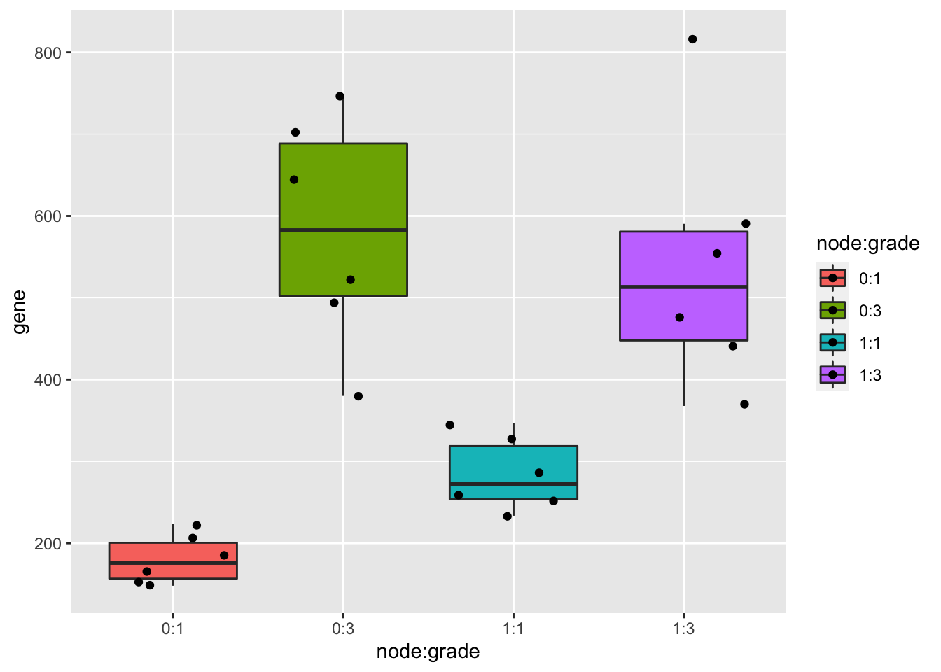

As discussed in a previous exercise, it seems that there is both an effect of histologic grade and lymph node status on the gene expression. There also seems to be a different effect of lymph node status on the gene expression for the different histologic grades.

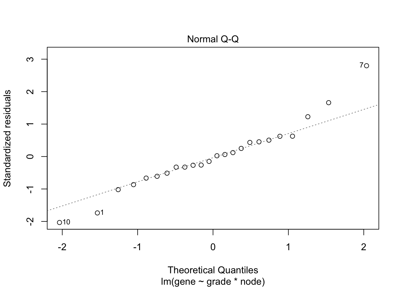
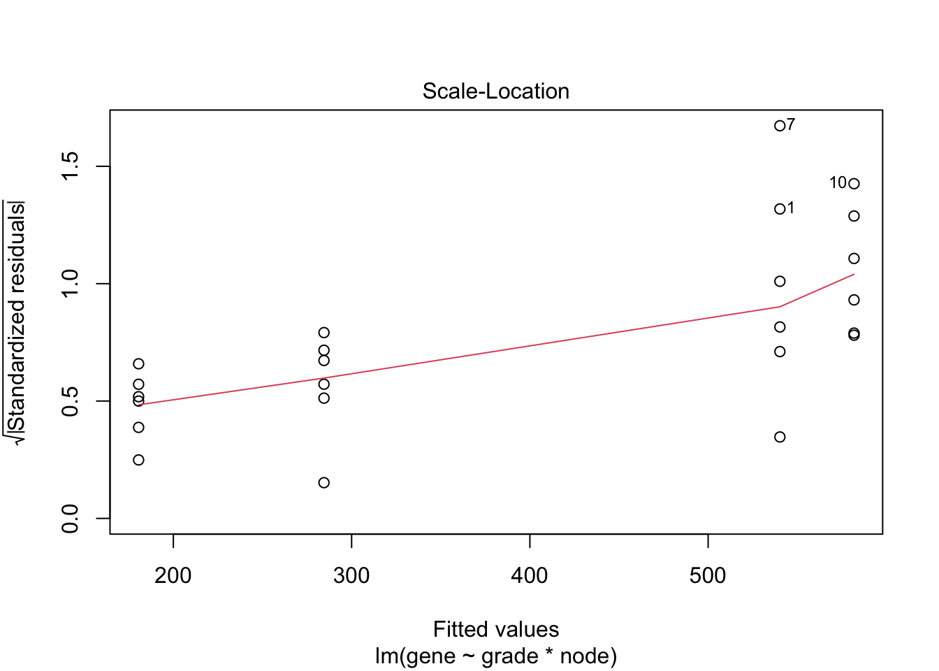
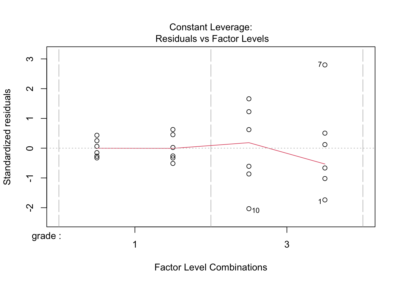
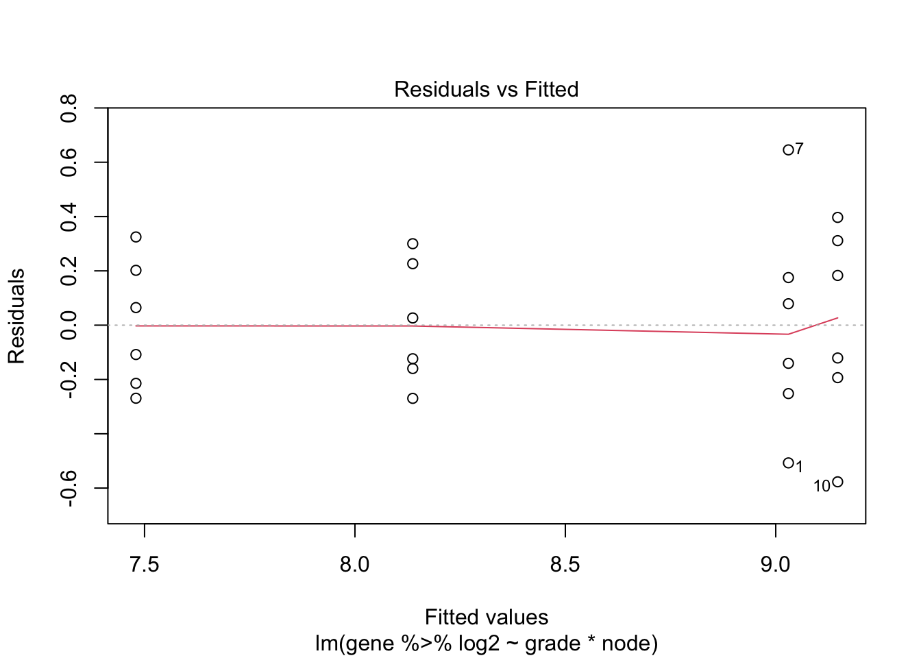
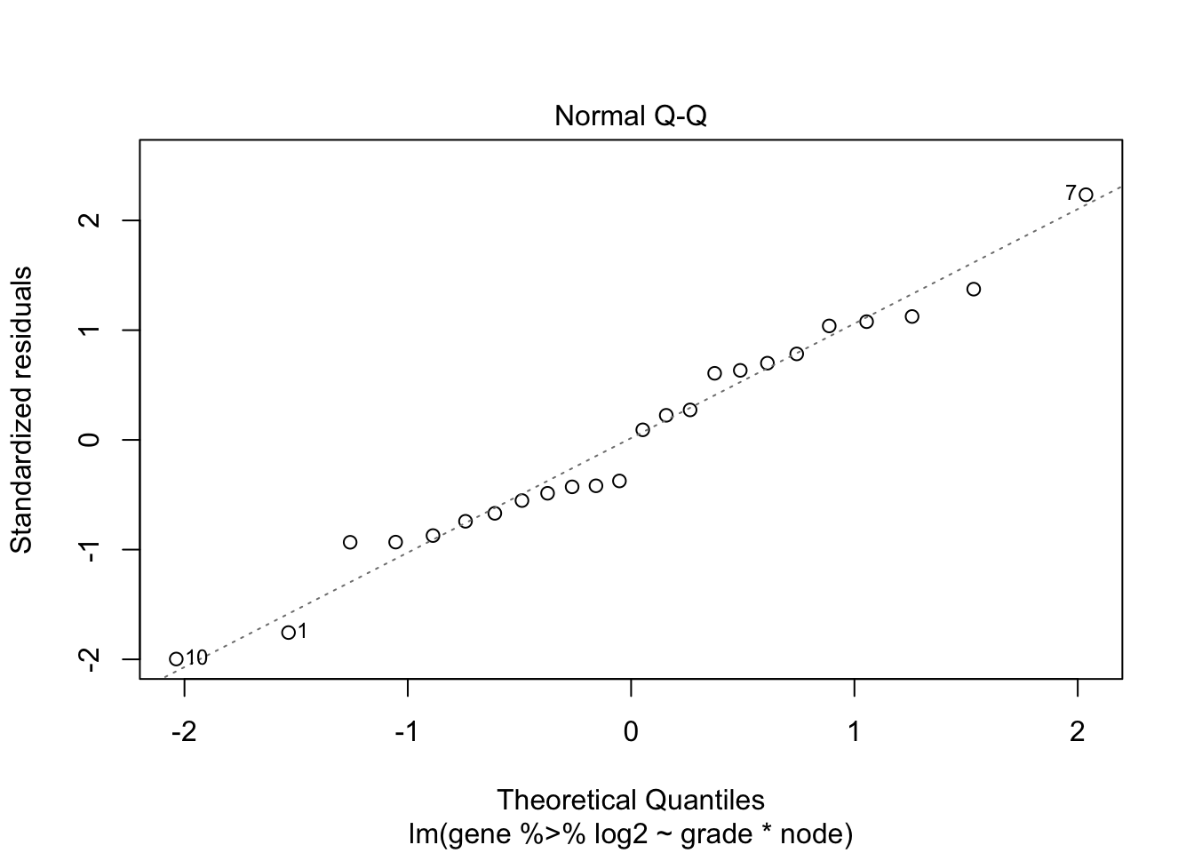
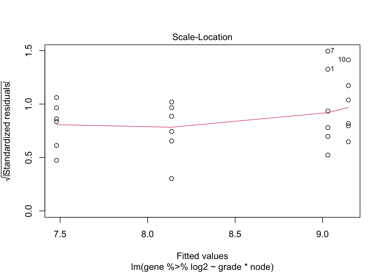
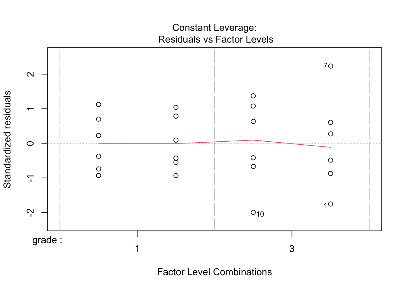
As we saw before, we can model this with a model that contains both histologic grade, lymph node status and the interaction term between both. When checking the linear model assumptions, we see that the variance is not equal. Therefore we model the gene expression with a log2-transformation, which makes that all the assumptions of the linear model are satisfied.

#Model with main effects for histological grade and node and grade x node interaction
fit <- lm(gene~grade*node,data=kpna2)
summary(fit)

## 
## Call:
## lm(formula = gene ~ grade * node, data = kpna2)
## 
## Residuals:
##      Min       1Q   Median       3Q      Max 
## -201.748  -53.294   -6.308   46.216  277.601 
## 
## Coefficients:
##              Estimate Std. Error t value Pr(>|t|)    
## (Intercept)    180.51      44.37   4.068   0.0006 ***
## grade3         401.33      62.75   6.396 3.07e-06 ***
## node1          103.98      62.75   1.657   0.1131    
## grade3:node1  -145.57      88.74  -1.640   0.1166    
## ---
## Signif. codes:  0 '***' 0.001 '**' 0.01 '*' 0.05 '.' 0.1 ' ' 1
## 
## Residual standard error: 108.7 on 20 degrees of freedom
## Multiple R-squared:  0.7437, Adjusted R-squared:  0.7052 
## F-statistic: 19.34 on 3 and 20 DF,  p-value: 3.971e-06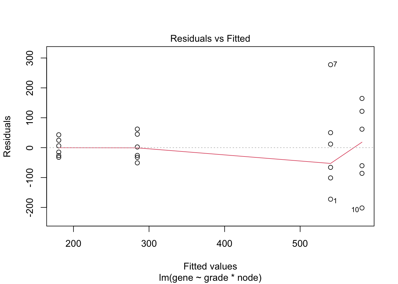

plot(fit)

fit <- lm(gene %>% log2~grade*node,data=kpna2)
plot(fit)

When checking the significance of the interaction term, we see that it is significant on the 5% significance level. We therefore keep the full model.

library(car)

## Loading required package: carData

## 
## Attaching package: 'car'

## The following object is masked from 'package:dplyr':
## 
##     recode

## The following object is masked from 'package:purrr':
## 
##     some

Anova(fit,type="III")

As we are dealing with a factorial design, we can calculate the mean gene expression for each group by the following parameter summations.

ExploreModelMatrix::VisualizeDesign(kpna2,~grade*node)$plotlist

## [[1]]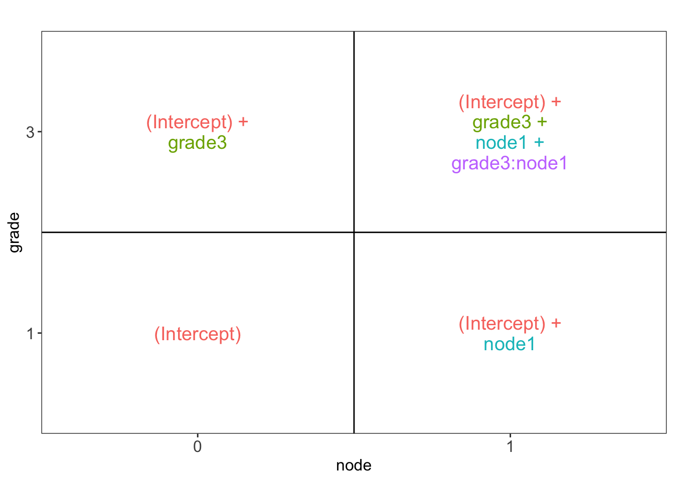

The researchers want to know the power for testing following hypotheses (remark that we will have to adjust for multiple testing):

• Log fold change between histologic grade 3 and histologic grade 1 for patients with unaffected lymph nodes (=0).

\[H_0: \log_2{FC}_{g3n0-g1n0} = \beta_{g3} = 0\]

• Log fold change between histologic grade 3 and histologic grade 1 for patients with removed lymph nodes (=1).

\[H_0: \log_2{FC}_{g3n1-g1n1} = \beta_{g3} + \beta_{g3n1} = 0\]

• Log fold change between unaffected and removed lymph nodes for patients of histologic grade 1.

\[H_0: \log_2{FC}_{g1n1-g1n0} = \beta_{n1} = 0\]

• Log fold change between unaffected and removed lymph nodes for patients of histologic grade 3.

\[H_0: \log_2{FC}_{g3n1-g3n0} = \beta_{n1} + \beta_{g3n1} = 0\]

• Difference in log fold change between patients of histological grade 3 and histological grade 1 with removed lymph nodes and log fold change between patients between patients of histological grade 3 and histological grade 1 with unaffected lymph nodes.

\[H_0: \log_2{FC}_{g3n1-g1n1} - \log_2{FC}_{g3n0-g1n0} = \beta_{g3n1} = 0\] which is an equivalent hypotheses with \[H_0: \log_2{FC}_{g3n1-g3n0} - \log_2{FC}_{g1n1-g1n0} = \beta_{g3n1} = 0\]

We can test this using multcomp, which controls for multiple testing.

library(multcomp)

## Loading required package: mvtnorm

## Loading required package: survival

## Loading required package: TH.data

## Loading required package: MASS

## 
## Attaching package: 'MASS'

## The following object is masked from 'package:dplyr':
## 
##     select

## 
## Attaching package: 'TH.data'

## The following object is masked from 'package:MASS':
## 
##     geyser

mcp <- glht(fit,linfct = c("grade3 = 0","grade3 + grade3:node1 = 0", "node1 = 0","node1 + grade3:node1 = 0", "grade3:node1 = 0"))
summary(mcp)

## 
##   Simultaneous Tests for General Linear Hypotheses
## 
## Fit: lm(formula = gene %>% log2 ~ grade * node, data = kpna2)
## 
## Linear Hypotheses:
##                            Estimate Std. Error t value Pr(>|t|)    
## grade3 == 0                  1.6675     0.1827   9.127  < 0.001 ***
## grade3 + grade3:node1 == 0   0.8928     0.1827   4.886  < 0.001 ***
## node1 == 0                   0.6577     0.1827   3.600  0.00711 ** 
## node1 + grade3:node1 == 0   -0.1170     0.1827  -0.640  0.89817    
## grade3:node1 == 0           -0.7748     0.2584  -2.998  0.02658 *  
## ---
## Signif. codes:  0 '***' 0.001 '**' 0.01 '*' 0.05 '.' 0.1 ' ' 1
## (Adjusted p values reported -- single-step method)

We get a significant p-value for the first, second, third and fifth hypothesis. The fourth hypothesis is not significant at the overall 5% significance level.

3 Power of the tests for each of the contrasts

3.1 Simulation function

Function to simulate data similar to that of our experiment under our model assumptions.

simFastMultipleContrasts <- function(form, data, betas, sd, contrasts, alpha = .05, nSim = 10000, adjust = "bonferroni")
{
    ySim <- rnorm(nrow(data)*nSim,sd=sd)
    dim(ySim) <-c(nrow(data),nSim)
    design <- model.matrix(form, data)
    ySim <- ySim + c(design %*%betas)
    ySim <- t(ySim)
  
    ### Fitting
    fitAll <- limma::lmFit(ySim,design)
  
    ### Inference
    varUnscaled <- t(contrasts)%*%fitAll$cov.coefficients%*%contrasts
    contrasts <- fitAll$coefficients %*%contrasts
    seContrasts <- matrix(diag(varUnscaled)^.5,nrow=nSim,ncol=5,byrow = TRUE)*fitAll$sigma
    tstats <- contrasts/seContrasts
    pvals <- pt(abs(tstats),fitAll$df.residual,lower.tail = FALSE)*2
    pvals <- t(apply(pvals, 1, p.adjust, method = adjust))
    
    return(colMeans(pvals < alpha))
}

3.2 power of current experiment

nSim <- 20000
betas <- fit$coefficients
sd <- sigma(fit)
contrasts <- matrix(0,nrow=4,ncol=5)
rownames(contrasts) <- names(fit$coefficients)
colnames(contrasts) <- c("graden0","graden1","nodeg1","nodeg3","interaction")
contrasts[2,1] <- 1
contrasts[c(2,4),2] <- 1
contrasts[3,3] <- 1
contrasts[c(3,4),4] <- 1
contrasts[4,5] <- 1
form <- ~ grade*node
power1 <- simFastMultipleContrasts(form, kpna2, betas, sd, contrasts, nSim = nSim)
power1

##     graden0     graden1      nodeg1      nodeg3 interaction 
##     1.00000     0.97005     0.76715     0.02380     0.57315

We observe large powers for all contrasts, except for contrast nodeg3, which has a small effect size.

3.3 Power for increasing sample size

nSim <- 20000
betas <- fit$coefficients
sd <- sigma(fit)
contrasts <- matrix(0,nrow=4,ncol=5)
rownames(contrasts) <- names(fit$coefficients)
colnames(contrasts) <- c("graden0","graden1","nodeg1","nodeg3","interaction")
contrasts[2,1] <- 1
contrasts[c(2,4),2] <- 1
contrasts[3,3] <- 1
contrasts[c(3,4),4] <- 1
contrasts[4,5] <- 1
form <- ~ grade*node

powers <- matrix(NA,nrow=9, ncol=6)
colnames(powers) <- c("n",colnames(contrasts))
powers[,1] <- 2:10

dataAllComb <- data.frame(grade = rep(c(1,3),each=2)%>% as.factor, 
                          node = rep(c(0,1),2)%>%as.factor) 
  
for (i in 1:nrow(powers))
{  
predData <- data.frame(grade = rep(dataAllComb$grade, powers[i,1]), 
                       node = rep(dataAllComb$node, powers[i,1]))
powers[i,-1] <- simFastMultipleContrasts(form, predData, betas, sd, contrasts, nSim = nSim)
}
powers

##        n graden0 graden1  nodeg1  nodeg3 interaction
##  [1,]  2 0.69955 0.20985 0.10980 0.01210     0.07100
##  [2,]  3 0.99265 0.56885 0.29765 0.01505     0.19005
##  [3,]  4 0.99990 0.80425 0.48150 0.01825     0.32385
##  [4,]  5 1.00000 0.92205 0.64395 0.02090     0.45290
##  [5,]  6 1.00000 0.96985 0.76520 0.02460     0.56785
##  [6,]  7 1.00000 0.99105 0.85340 0.02775     0.66360
##  [7,]  8 1.00000 0.99640 0.90625 0.03030     0.75270
##  [8,]  9 1.00000 0.99905 0.94405 0.03495     0.81640
##  [9,] 10 1.00000 0.99960 0.96950 0.03805     0.87120

powers %>% 
  as.data.frame %>% 
  gather(contrast, power, -n) %>% 
  ggplot(aes(n,power,color=contrast)) +
  geom_line()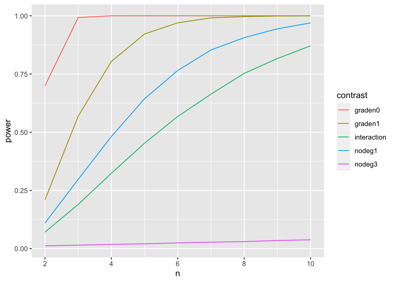

3.4 Power when FC for grade in patients with unaffected lymph nodes equals 1.5 (\(\beta_g\) = 1.5)

nSim <- 20000
betas2 <- fit$coefficients
betas2["grade3"] <- log2(1.5)
sd <- sigma(fit)
contrasts <- matrix(0,nrow=4,ncol=5)
rownames(contrasts) <- names(fit$coefficients)
colnames(contrasts) <- c("graden0","graden1","nodeg1","nodeg3","interaction")
contrasts[2,1] <- 1
contrasts[c(2,4),2] <- 1
contrasts[3,3] <- 1
contrasts[c(3,4),4] <- 1
contrasts[4,5] <- 1
form <- ~ grade*node
power3 <- simFastMultipleContrasts(form, kpna2, betas2, sd, contrasts,nSim = nSim)
power3

##     graden0     graden1      nodeg1      nodeg3 interaction 
##     0.64100     0.05465     0.76170     0.02465     0.56510

It is clear that only the power of the contrasts containing \(\beta_g\) change when the effect size of \(\beta_g\) changes.

---

This work is licensed under the CC BY-NC-SA 4.0 licence.