1. Introduction: Linear Regression - Geometric interpretation

1 Intro

1.1 Data

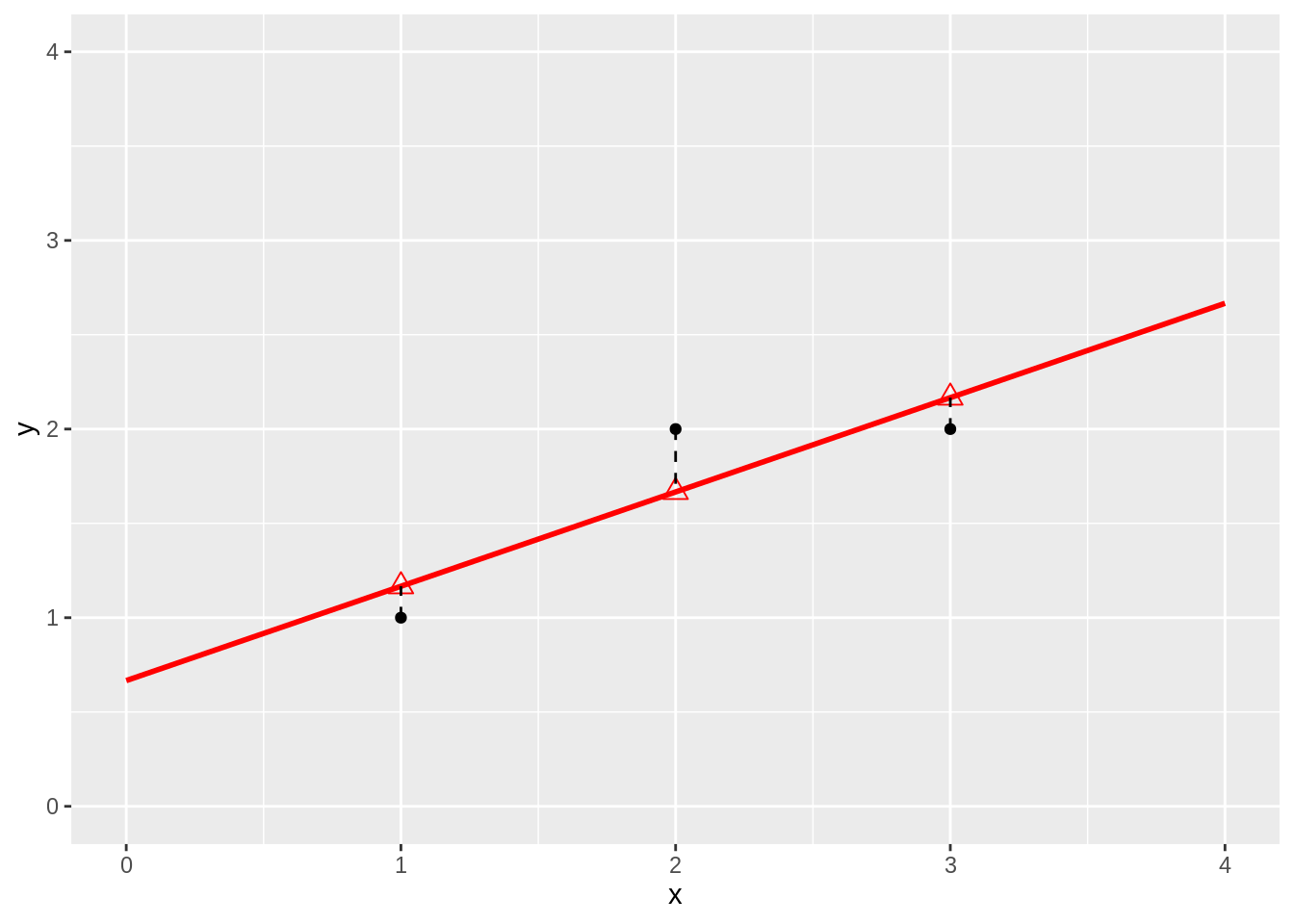
Dataset with 3 observation (X,Y):

library(tidyverse)

## ── Attaching packages ─────────────────────────────────────── tidyverse 1.3.1 ──

## ✔ ggplot2 3.3.5     ✔ purrr   0.3.4
## ✔ tibble  3.1.5     ✔ dplyr   1.0.7
## ✔ tidyr   1.1.4     ✔ stringr 1.4.0
## ✔ readr   2.0.1     ✔ forcats 0.5.1

## ── Conflicts ────────────────────────────────────────── tidyverse_conflicts() ──
## ✖ dplyr::filter() masks stats::filter()
## ✖ dplyr::lag()    masks stats::lag()

data <- data.frame(x=1:3,y=c(1,2,2))
data

1.2 Model

\[ y_i=\beta_0+\beta_1x + \epsilon_i \]

If we write the model for each observation:

\[ \begin{array} {lcl} 1 &=& \beta_0+\beta_1 1 + \epsilon_1 \\ 2 &=& \beta_0+\beta_1 2 + \epsilon_2 \\ 2 &=& \beta_0+\beta_1 2 + \epsilon_3 \\ \end{array} \]

We can also write this in matrix form

\[ \mathbf{Y} = \mathbf{X}\boldsymbol{\beta}+\boldsymbol{\epsilon} \]

with

\[ \mathbf{Y}=\left[ \begin{array}{c} 1\\ 2\\ 2\\ \end{array}\right], \quad \mathbf{X}= \left[ \begin{array}{cc} 1&1\\ 1&2\\ 1&3\\ \end{array} \right], \quad \boldsymbol{\beta} = \left[ \begin{array}{c} \beta_0\\ \beta_1\\ \end{array} \right] \quad \text{and} \quad \boldsymbol{\epsilon}= \left[ \begin{array}{c} \epsilon_1\\ \epsilon_2\\ \epsilon_3 \end{array} \right] \]

lm1 <- lm(y~x,data)
data$yhat <- lm1$fitted

data %>%
  ggplot(aes(x,y)) +
  geom_point() +
  ylim(0,4) +
  xlim(0,4) +
  stat_smooth(method = "lm", color = "red", fullrange = TRUE) +
  geom_point(aes(x=x, y =yhat), pch = 2, size = 3, color = "red") +
  geom_segment(data = data, aes(x = x, xend = x, y = y, yend = yhat), lty = 2 )

## `geom_smooth()` using formula 'y ~ x'

## Warning in max(ids, na.rm = TRUE): no non-missing arguments to max; returning
## -Inf

2 Least Squares (LS)

• Minimize the residual sum of squares \[\begin{eqnarray*} RSS(\boldsymbol{\beta})&=&\sum\limits_{i=1}^n e^2_i\\ &=&\sum\limits_{i=1}^n \left(y_i-\beta_0-\sum\limits_{j=1}^p x_{ij}\beta_j\right)^2 \end{eqnarray*}\]

• or in matrix notation \[\begin{eqnarray*} RSS(\boldsymbol{\beta})&=&(\mathbf{Y}-\mathbf{X\beta})^T(\mathbf{Y}-\mathbf{X\beta})\\ &=&\Vert \mathbf{Y}-\mathbf{X\beta}\Vert^2_2 \end{eqnarray*}\] with the \(L_2\)-norm of a \(p\)-dim. vector \(v\) \(\Vert \mathbf{v} \Vert_2=\sqrt{v_1^2+\ldots+v_p^2}\) \(\rightarrow\) \(\hat{\boldsymbol{\beta}}=\text{argmin}_\beta \Vert \mathbf{Y}-\mathbf{X\beta}\Vert^2\)

2.1 Minimize RSS

\[ \begin{array}{ccc} \frac{\partial RSS}{\partial \boldsymbol{\beta}}&=&\mathbf{0}\\\\ \frac{(\mathbf{Y}-\mathbf{X\beta})^T(\mathbf{Y}-\mathbf{X}\boldsymbol{\beta})}{\partial \boldsymbol{\beta}}&=&\mathbf{0}\\\\ -2\mathbf{X}^T(\mathbf{Y}-\mathbf{X}\boldsymbol{\beta})&=&\mathbf{0}\\\\ \mathbf{X}^T\mathbf{X\beta}&=&\mathbf{X}^T\mathbf{Y}\\\\ \hat{\boldsymbol{\beta}}&=&(\mathbf{X}^T\mathbf{X})^{-1}\mathbf{X}^T\mathbf{Y} \end{array} \]

\[ \hat{\boldsymbol{\beta}}=(\mathbf{X}^T\mathbf{X})^{-1}\mathbf{X}^T\mathbf{Y} \]

2.2 Fitted values:

\[ \begin{array}{lcl} \hat{\mathbf{Y}} &=& \mathbf{X}\hat{\boldsymbol{\beta}}\\ &=& \mathbf{X} (\mathbf{X}^T\mathbf{X})^{-1}\mathbf{X}^T\mathbf{Y}\\ \end{array} \]

3 Geometric interpretation of Linear regression

There is also another picture to interpret linear regression!

Linear regression can also be seen as a projection!

Fitted values:

\[ \begin{array}{lcl} \hat{\mathbf{Y}} &=& \mathbf{X}\hat{\boldsymbol{\beta}}\\ &=& \mathbf{X} (\mathbf{X}^T\mathbf{X})^{-1}\mathbf{X}^T\mathbf{Y}\\ &=& \mathbf{HY} \end{array} \] with \(\mathbf{H}\) the projection matrix also referred to as the hat matrix.

X <- model.matrix(~x,data)
X

##   (Intercept) x
## 1           1 1
## 2           1 2
## 3           1 3
## attr(,"assign")
## [1] 0 1

XtX <- t(X)%*%X
XtX

##             (Intercept)  x
## (Intercept)           3  6
## x                     6 14

XtXinv <- solve(t(X)%*%X)
XtXinv

##             (Intercept)    x
## (Intercept)    2.333333 -1.0
## x             -1.000000  0.5

H <- X %*% XtXinv %*% t(X)
H

##            1         2          3
## 1  0.8333333 0.3333333 -0.1666667
## 2  0.3333333 0.3333333  0.3333333
## 3 -0.1666667 0.3333333  0.8333333

Y <- data$y
Yhat <- H%*%Y
Yhat

##       [,1]
## 1 1.166667
## 2 1.666667
## 3 2.166667

3.1 What do these projections mean geometrically?

The other picture to linear regression is to consider \(X_0\), \(X_1\) and \(Y\) as vectors in the space of the data \(\mathbb{R}^n\), here \(\mathbb{R}^3\) because we have three data points.

originRn <- data.frame(X1=0,X2=0,X3=0)
data$x0 <- 1
dataRn <- data.frame(t(data))

library(plotly)

## 
## Attaching package: 'plotly'

## The following object is masked from 'package:ggplot2':
## 
##     last_plot

## The following object is masked from 'package:stats':
## 
##     filter

## The following object is masked from 'package:graphics':
## 
##     layout

p1 <- plot_ly(
    originRn,
    x = ~ X1,
    y = ~ X2,
    z= ~ X3) %>%
  add_markers(type="scatter3d") %>%
  layout(
    scene = list(
      aspectmode="cube",
      xaxis = list(range=c(-4,4)), yaxis = list(range=c(-4,4)), zaxis = list(range=c(-4,4))
      )
    )
p1 <- p1 %>%
  add_trace(
    x = c(0,1),
    y = c(0,0),
    z = c(0,0),
    mode = "lines",
    line = list(width = 5, color = "grey"),
    type="scatter3d") %>%
  add_trace(
    x = c(0,0),
    y = c(0,1),
    z = c(0,0),
    mode = "lines",
    line = list(width = 5, color = "grey"),
    type="scatter3d") %>%
  add_trace(
    x = c(0,0),
    y = c(0,0),
    z = c(0,1),
    mode = "lines",
    line = list(width = 5, color = "grey"),
    type="scatter3d") %>%
  add_trace(
    x = c(0,1),
    y = c(0,1),
    z = c(0,1),
    mode = "lines",
    line = list(width = 5, color = "black"),
    type="scatter3d") %>%
    add_trace(
    x = c(0,1),
    y = c(0,2),
    z = c(0,3),
    mode = "lines",
    line = list(width = 5, color = "black"),
    type="scatter3d")

p2 <- p1 %>%
  add_trace(
    x = c(0,Y[1]),
    y = c(0,Y[2]),
    z = c(0,Y[3]),
    mode = "lines",
    line = list(width = 5, color = "red"),
    type="scatter3d") %>%
  add_trace(
    x = c(0,Yhat[1]),
    y = c(0,Yhat[2]),
    z = c(0,Yhat[3]),
    mode = "lines",
    line = list(width = 5, color = "red"),
    type="scatter3d") %>% add_trace(
    x = c(Y[1],Yhat[1]),
    y = c(Y[2],Yhat[2]),
    z = c(Y[3],Yhat[3]),
    mode = "lines",
    line = list(width = 5, color = "red", dash="dash"),
    type="scatter3d")
p2

3.1.1 How does this projection work?

\[ \begin{array}{lcl} \hat{\mathbf{Y}} &=& \mathbf{X} (\mathbf{X}^T\mathbf{X})^{-1}\mathbf{X}^T\mathbf{Y}\\ &=& \mathbf{X}(\mathbf{X}^T\mathbf{X})^{-1/2}(\mathbf{X}^T\mathbf{X})^{-1/2}\mathbf{X}^T\mathbf{Y}\\ &=& \mathbf{U}\mathbf{U}^T\mathbf{Y} \end{array} \]

• \(\mathbf{U}\) is a new orthonormal basis in \(\mathbb{R}^2\), a subspace of \(\mathbb{R}^3\)

• The space spanned by U and X is the column space of X, e.g. it contains all possible linear combinantions of X. \(\mathbf{U}^t\mathbf{Y}\) is the projection of Y on this new orthonormal basis

eigenXtX <- eigen(XtX)
XtXinvSqrt <- eigenXtX$vectors %*%diag(1/eigenXtX$values^.5)%*%t(eigenXtX$vectors)
U <- X %*% XtXinvSqrt

p3 <- p1 %>%
  add_trace(
    x = c(0,U[1,1]),
    y = c(0,U[2,1]),
    z = c(0,U[3,1]),
    mode = "lines",
    line = list(width = 5, color = "blue"),
    type="scatter3d") %>%
  add_trace(
    x = c(0,U[1,2]),
    y = c(0,U[2,2]),
    z = c(0,U[3,2]),
    mode = "lines",
    line = list(width = 5, color = "blue"),
    type="scatter3d")

p3

• \(\mathbf{U}^T\mathbf{Y}\) is the projection of \(\mathbf{Y}\) in the space spanned by \(\mathbf{U}\).
• Indeed \(\mathbf{U}_1^T\mathbf{Y}\)

p4 <- p3 %>%
  add_trace(
    x = c(0,Y[1]),
    y = c(0,Y[2]),
    z = c(0,Y[3]),
    mode = "lines",
    line = list(width = 5, color = "red"),
    type="scatter3d") %>%
  add_trace(
    x = c(0,U[1,1]*(U[,1]%*%Y)),
    y = c(0,U[2,1]*(U[,1]%*%Y)),
    z = c(0,U[3,1]*(U[,1]%*%Y)),
    mode = "lines",
    line = list(width = 5, color = "red",dash="dash"),
    type="scatter3d") %>% add_trace(
    x = c(Y[1],U[1,1]*(U[,1]%*%Y)),
    y = c(Y[2],U[2,1]*(U[,1]%*%Y)),
    z = c(Y[3],U[3,1]*(U[,1]%*%Y)),
    mode = "lines",
    line = list(width = 5, color = "red", dash="dash"),
    type="scatter3d")
p4

• and \(\mathbf{U}_2^T\mathbf{Y}\)

p5 <- p4 %>%
  add_trace(
    x = c(0,Y[1]),
    y = c(0,Y[2]),
    z = c(0,Y[3]),
    mode = "lines",
    line = list(width = 5, color = "red"),
    type="scatter3d") %>%
  add_trace(
    x = c(0,U[1,2]*(U[,2]%*%Y)),
    y = c(0,U[2,2]*(U[,2]%*%Y)),
    z = c(0,U[3,2]*(U[,2]%*%Y)),
    mode = "lines",
    line = list(width = 5, color = "red",dash="dash"),
    type="scatter3d") %>% add_trace(
    x = c(Y[1],U[1,2]*(U[,2]%*%Y)),
    y = c(Y[2],U[2,2]*(U[,2]%*%Y)),
    z = c(Y[3],U[3,2]*(U[,2]%*%Y)),
    mode = "lines",
    line = list(width = 5, color = "red", dash="dash"),
    type="scatter3d")
p5

p6 <- p5 %>%
  add_trace(
    x = c(0,Yhat[1]),
    y = c(0,Yhat[2]),
    z = c(0,Yhat[3]),
    mode = "lines",
    line = list(width = 5, color = "red"),
    type="scatter3d") %>%
  add_trace(
    x = c(Y[1],Yhat[1]),
    y = c(Y[2],Yhat[2]),
    z = c(Y[3],Yhat[3]),
    mode = "lines",
    line = list(width = 5, color = "red", dash="dash"),
    type="scatter3d") %>%
  add_trace(
    x = c(U[1,1]*(U[,1]%*%Y),Yhat[1]),
    y = c(U[2,1]*(U[,1]%*%Y),Yhat[2]),
    z = c(U[3,1]*(U[,1]%*%Y),Yhat[3]),
    mode = "lines",
    line = list(width = 5, color = "red", dash="dash"),
    type="scatter3d")  %>%
  add_trace(
    x = c(U[1,2]*(U[,2]%*%Y),Yhat[1]),
    y = c(U[2,2]*(U[,2]%*%Y),Yhat[2]),
    z = c(U[3,2]*(U[,2]%*%Y),Yhat[3]),
    mode = "lines",
    line = list(width = 5, color = "red", dash="dash"),
    type="scatter3d")
p6

3.2 The Error vector

Note, that it is also clear from the equation in the derivation of the least squares solution that the residual is orthogonal on the column space:

\[ -2 \mathbf{X}^T(\mathbf{Y}-\mathbf{X}\boldsymbol{\beta}) = 0 \]

4 Curse of dimensionality?

• Imagine what happens when p approaches n \(p=n\) or becomes much larger than p >> n!!!

• Suppose that we add a predictor \(\mathbf{X}_2 = [2,0,1]^T\)?

\[ \mathbf{Y}=\left[ \begin{array}{c} 1\\ 2\\ 2\\ \end{array}\right], \quad \mathbf{X}= \left[ \begin{array}{ccc} 1&1&2\\ 1&2&0\\ 1&3&1\\ \end{array} \right], \quad \boldsymbol{\beta} = \left[ \begin{array}{c} \beta_0\\ \beta_1\\ \beta_2 \end{array} \right] \quad \text{and} \quad \boldsymbol{\epsilon}= \left[ \begin{array}{c} \epsilon_1\\ \epsilon_2\\ \epsilon_3 \end{array} \right] \]

data$x2 <- c(2,0,1)
fit <- lm(y~x+x2,data)
# predict values on regular xy grid
x1pred <- seq(-1, 4, length.out = 10)
x2pred <- seq(-1, 4, length.out = 10)
xy <- expand.grid(x = x1pred,
x2 = x2pred)
ypred <- matrix (nrow = 30, ncol = 30,
data = predict(fit, newdata = data.frame(xy)))

library(plot3D)

## Warning: no DISPLAY variable so Tk is not available

# fitted points for droplines to surface
th=20
ph=5
scatter3D(data$x,
  data$x2,
  Y,
  pch = 16,
  col="darkblue",
  cex = 1,
  theta = th,
  ticktype = "detailed",
  xlab = "x1",
  ylab = "x2",
  zlab = "y",
  colvar=FALSE,
  bty = "g",
  xlim=c(-1,3),
  ylim=c(-1,3),
  zlim=c(-2,4))

z.pred3D <- outer(
  x1pred,
  x2pred,
  function(x1,x2)
  {
    fit$coef[1] + fit$coef[2]*x1+fit$coef[2]*x2
  })

x.pred3D <- outer(
  x1pred,
  x2pred,
  function(x,y) x)

y.pred3D <- outer(
  x1pred,
  x2pred,
  function(x,y) y)

scatter3D(data$x,
  data$x2,
  data$y,
  pch = 16,
  col="darkblue",
  cex = 1,
  theta = th,
  ticktype = "detailed",
  xlab = "x1",
  ylab = "x2",
  zlab = "y",
  colvar=FALSE,
  bty = "g",
  xlim=c(-1,4),
  ylim=c(-1,4),
  zlim=c(-2,4))

surf3D(
  x.pred3D,
  y.pred3D,
  z.pred3D,
  col="blue",
  facets=NA,
  add=TRUE)

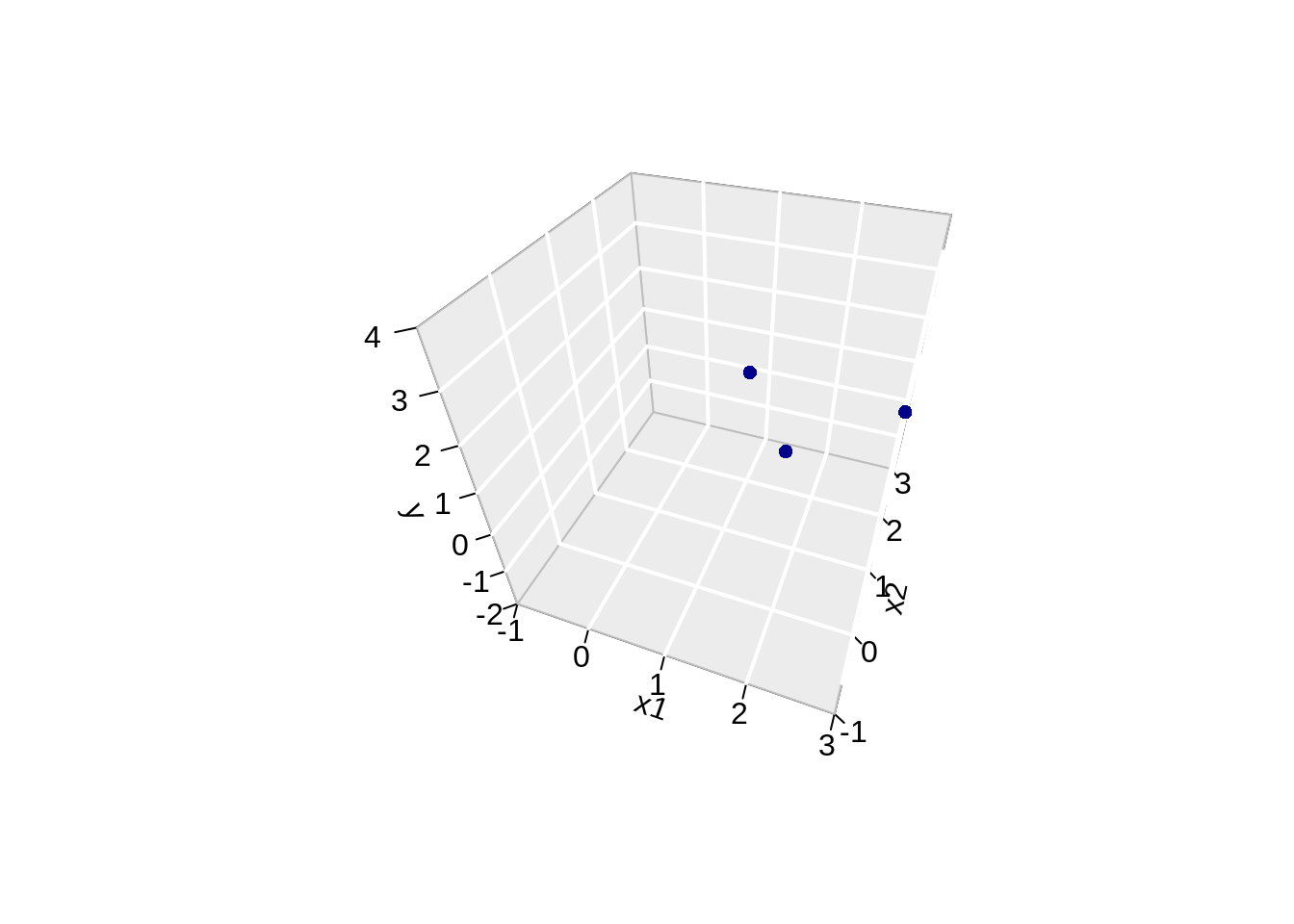
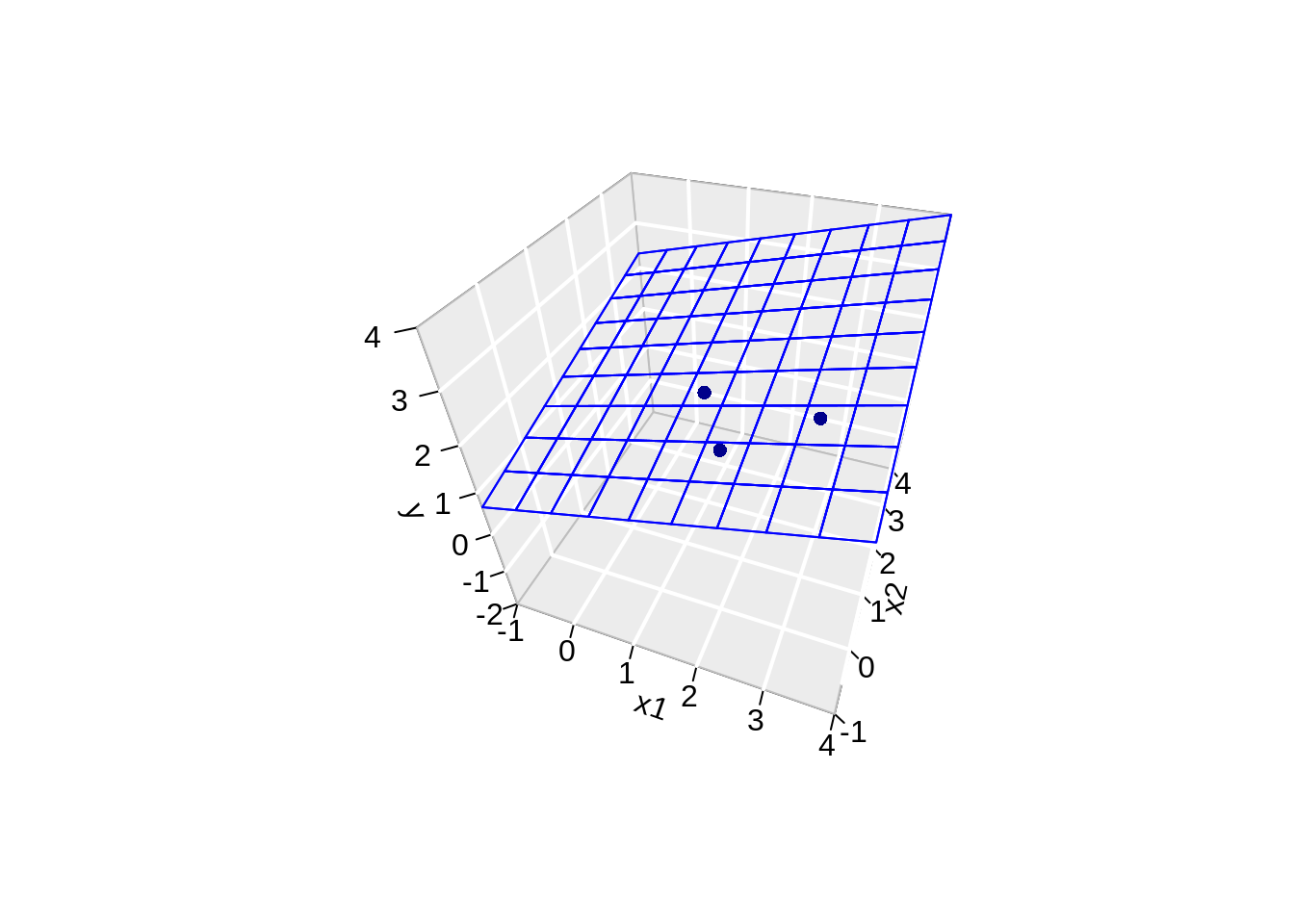
Note, that the linear regression is now a plane.

However, we obtain a perfect fit and all the data points are falling in the plane! 😱

This is obvious if we look at the column space of X!

X <- cbind(X,c(2,0,1))
XtX <- t(X)%*%X
eigenXtX <- eigen(XtX)
XtXinvSqrt <- eigenXtX$vectors %*%diag(1/eigenXtX$values^.5)%*%t(eigenXtX$vectors)
U <- X %*% XtXinvSqrt

p7 <- p1 %>%
  add_trace(
    x = c(0,2),
    y = c(0,0),
    z = c(0,1),
    mode = "lines",
    line = list(width = 5, color = "darkgreen"),
    type="scatter3d")
p7

p8 <- p7 %>%
  add_trace(
    x = c(0,U[1,1]),
    y = c(0,U[2,1]),
    z = c(0,U[3,1]),
    mode = "lines",
    line = list(width = 5, color = "blue"),
    type="scatter3d") %>%
  add_trace(
    x = c(0,U[1,2]),
    y = c(0,U[2,2]),
    z = c(0,U[3,2]),
    mode = "lines",
    line = list(width = 5, color = "blue"),
    type="scatter3d") %>%
  add_trace(
    x = c(0,U[1,3]),
    y = c(0,U[2,3]),
    z = c(0,U[3,3]),
    mode = "lines",
    line = list(width = 5, color = "blue"),
    type="scatter3d")

p8

• The column space now spans the entire \(\mathbb{R}^3\)!

• With the intercept and the two predictors we can thus fit every dataset that only has 3 observations for the predictors and the response.

• So the model can no longer be used to generalise the patterns seen in the data towards the population (new observations).

• Problem of overfitting!!!

• If \(p >> n\) then the problem gets even worse! Then there is even no longer a unique solution to the least squares problem…

---

This work is licensed under the CC BY-NC-SA 4.0 licence.