Lab 1: Introduction and Singular Value Decomposition

High Dimensional Data Analysis practicals

Change log

---

1 Introduction

The purpose of the following exercises is mainly to get more familiar with SVD and its applications, in particular Multidimensional Scaling (MDS). It is recommended to perform the exercises in an RMarkdown document.

For a brief introduction to RMarkdown, see Introduction to RMarkdown.

For an introduction to working with matrices in R, see Working with Matrices in R.

Libraries

Packages used in this document. Installation code is commented, uncomment and paste this code in an R console to install the packages.

## Install necessary packages with:
# install.packages("tidyverse")
# if (!requireNamespace("remotes", quietly = TRUE)) {
#     install.packages("remotes")
# }
# remotes::install_github("statOmics/HDDAData")

library(tidyverse)
library(HDDAData)

2 Multidimensional Scaling (MDS) demonstration

See course notes for background.

• We will use UScitiesD data as an example
• Our goal is to use the distance matrix \(\mathbf D_X\) without knowledge of \(\mathbf X\) to represent the rows of \(\mathbf X\) in a low dimensional space, say 2D or 3D.
• We search for \(\mathbf V_k\) that orthogonally projects the rows of \(\mathbf X\) (\(\mathbf x^T_i\)) onto a \(k\)-dimensional space spanned by the columns of \(\mathbf V_k\). In fact we are looking for \(\mathbf Z_k\), such that \(\mathbf Z_k=\mathbf X \mathbf V_k\)
• But we do not know \(\mathbf X\), so how do we get \(\mathbf Z_k\)? We will use the \(\mathbf G_X\) (gram matrix) trick, mentioned in the course notes

2.1 Example: Distances between US cities

As an example, we will use the UScitiesD data set, which is part of base R. This data gives “straight line” distances (in km) between 10 cities in the US.

UScitiesD
#>               Atlanta Chicago Denver Houston LosAngeles Miami NewYork SanFrancisco Seattle
#> Chicago           587                                                                     
#> Denver           1212     920                                                             
#> Houston           701     940    879                                                      
#> LosAngeles       1936    1745    831    1374                                              
#> Miami             604    1188   1726     968       2339                                   
#> NewYork           748     713   1631    1420       2451  1092                             
#> SanFrancisco     2139    1858    949    1645        347  2594    2571                     
#> Seattle          2182    1737   1021    1891        959  2734    2408          678        
#> Washington.DC     543     597   1494    1220       2300   923     205         2442    2329

class(UScitiesD)
#> [1] "dist"

Note that the UScitiesD object is of class "dist", which is a special type of object to represent that it is a distance matrix (we’ll denote this as \(\mathbf{D}_X\)), i.e. the result from computing distances from an original matrix \(\mathbf{X}\). In this case, the original matrix \(\mathbf{X}\) was likely a matrix with a row for every city and columns specifying its coordinates. Note though that we don’t know \(\mathbf{X}\) exactly. Still, we can use the distance matrix and MDS to approximate a low-dimensional representation of \(\mathbf{X}\).

2.1.1 Exploring the distance matrix

We first convert the UScitiesD to a matrix for easier manipulation and calculation. Note that this creates a “symmetrical” matrix, with 0s on the diagonal (distance of a city to itself).

(dist_mx <- as.matrix(UScitiesD))
#>               Atlanta Chicago Denver Houston LosAngeles Miami NewYork
#> Atlanta             0     587   1212     701       1936   604     748
#> Chicago           587       0    920     940       1745  1188     713
#> Denver           1212     920      0     879        831  1726    1631
#> Houston           701     940    879       0       1374   968    1420
#> LosAngeles       1936    1745    831    1374          0  2339    2451
#> Miami             604    1188   1726     968       2339     0    1092
#> NewYork           748     713   1631    1420       2451  1092       0
#> SanFrancisco     2139    1858    949    1645        347  2594    2571
#> Seattle          2182    1737   1021    1891        959  2734    2408
#> Washington.DC     543     597   1494    1220       2300   923     205
#>               SanFrancisco Seattle Washington.DC
#> Atlanta               2139    2182           543
#> Chicago               1858    1737           597
#> Denver                 949    1021          1494
#> Houston               1645    1891          1220
#> LosAngeles             347     959          2300
#> Miami                 2594    2734           923
#> NewYork               2571    2408           205
#> SanFrancisco             0     678          2442
#> Seattle                678       0          2329
#> Washington.DC         2442    2329             0

The dimensions of dist_mx:

# 10 x 10 square matrix
dim(dist_mx)
#> [1] 10 10

And the rank of dist_mx

qr(dist_mx)$rank
#> [1] 10

Q: is this matrix of full rank?

Answer

A: Yes, it is.

qr(dist_mx)$rank == min(dim(dist_mx))
#> [1] TRUE

2.1.2 \(\mathbf{H}\) and \(\mathbf{G}_X\) matrices

Now let’s create the \(\mathbf H\) matrix.

\[ \mathbf{H} = \mathbf{I}_{n \times n} - \frac{1}{n} \mathbf{1}_n\mathbf{1}_n^T \]

n <- nrow(dist_mx)

## 11^T
## Alternatively: one_mat <- rep(1, n) %o% rep(1, n)
(one_mat <- matrix(rep(1, n * n), ncol = n, nrow = n))
#>       [,1] [,2] [,3] [,4] [,5] [,6] [,7] [,8] [,9] [,10]
#>  [1,]    1    1    1    1    1    1    1    1    1     1
#>  [2,]    1    1    1    1    1    1    1    1    1     1
#>  [3,]    1    1    1    1    1    1    1    1    1     1
#>  [4,]    1    1    1    1    1    1    1    1    1     1
#>  [5,]    1    1    1    1    1    1    1    1    1     1
#>  [6,]    1    1    1    1    1    1    1    1    1     1
#>  [7,]    1    1    1    1    1    1    1    1    1     1
#>  [8,]    1    1    1    1    1    1    1    1    1     1
#>  [9,]    1    1    1    1    1    1    1    1    1     1
#> [10,]    1    1    1    1    1    1    1    1    1     1

## Calculate H, diag(n) is the nxn identity matrix
(H <- diag(n) - (1/n) * one_mat)
#>       [,1] [,2] [,3] [,4] [,5] [,6] [,7] [,8] [,9] [,10]
#>  [1,]  0.9 -0.1 -0.1 -0.1 -0.1 -0.1 -0.1 -0.1 -0.1  -0.1
#>  [2,] -0.1  0.9 -0.1 -0.1 -0.1 -0.1 -0.1 -0.1 -0.1  -0.1
#>  [3,] -0.1 -0.1  0.9 -0.1 -0.1 -0.1 -0.1 -0.1 -0.1  -0.1
#>  [4,] -0.1 -0.1 -0.1  0.9 -0.1 -0.1 -0.1 -0.1 -0.1  -0.1
#>  [5,] -0.1 -0.1 -0.1 -0.1  0.9 -0.1 -0.1 -0.1 -0.1  -0.1
#>  [6,] -0.1 -0.1 -0.1 -0.1 -0.1  0.9 -0.1 -0.1 -0.1  -0.1
#>  [7,] -0.1 -0.1 -0.1 -0.1 -0.1 -0.1  0.9 -0.1 -0.1  -0.1
#>  [8,] -0.1 -0.1 -0.1 -0.1 -0.1 -0.1 -0.1  0.9 -0.1  -0.1
#>  [9,] -0.1 -0.1 -0.1 -0.1 -0.1 -0.1 -0.1 -0.1  0.9  -0.1
#> [10,] -0.1 -0.1 -0.1 -0.1 -0.1 -0.1 -0.1 -0.1 -0.1   0.9

We can use \(\mathbf{H}\) to center our distance matrix:

(dist_mx_centered <- H %*% dist_mx)
#>       Atlanta Chicago  Denver Houston LosAngeles   Miami NewYork SanFrancisco
#>  [1,] -1065.2  -441.5   145.7  -402.8      507.8  -812.8  -575.9        616.7
#>  [2,]  -478.2 -1028.5  -146.3  -163.8      316.8  -228.8  -610.9        335.7
#>  [3,]   146.8  -108.5 -1066.3  -224.8     -597.2   309.2   307.1       -573.3
#>  [4,]  -364.2   -88.5  -187.3 -1103.8      -54.2  -448.8    96.1        122.7
#>  [5,]   870.8   716.5  -235.3   270.2    -1428.2   922.2  1127.1      -1175.3
#>  [6,]  -461.2   159.5   659.7  -135.8      910.8 -1416.8  -231.9       1071.7
#>  [7,]  -317.2  -315.5   564.7   316.2     1022.8  -324.8 -1323.9       1048.7
#>  [8,]  1073.8   829.5  -117.3   541.2    -1081.2  1177.2  1247.1      -1522.3
#>  [9,]  1116.8   708.5   -45.3   787.2     -469.2  1317.2  1084.1       -844.3
#> [10,]  -522.2  -431.5   427.7   116.2      871.8  -493.8 -1118.9        919.7
#>       Seattle Washington.DC
#>  [1,]   588.1        -662.3
#>  [2,]   143.1        -608.3
#>  [3,]  -572.9         288.7
#>  [4,]   297.1          14.7
#>  [5,]  -634.9        1094.7
#>  [6,]  1140.1        -282.3
#>  [7,]   814.1       -1000.3
#>  [8,]  -915.9        1236.7
#>  [9,] -1593.9        1123.7
#> [10,]   735.1       -1205.3

## Verify colMeans are 0
round(colMeans(dist_mx_centered), 8)
#>       Atlanta       Chicago        Denver       Houston    LosAngeles 
#>             0             0             0             0             0 
#>         Miami       NewYork  SanFrancisco       Seattle Washington.DC 
#>             0             0             0             0             0

## Note that using `scale(X, center = TRUE, scale = FALSE)` is much more efficient
## to center a matrix
## Here we use the approach with H because we need it further on

We will use this matrix to calculate \(\mathbf{G}_X\) (Gram matrix of \(\mathbf{X}\)).

\[ \mathbf{G}_X = -\frac{1}{2}\mathbf{H}\mathbf{D}_X\mathbf{H} = \mathbf{X}\mathbf{X}^T \]

Where \(\mathbf{D}_X\) is the matrix of squared distances. So we will first have to square our dist_mx.

## D_X = squared distance matrix
D_X <- dist_mx ^ 2

## Gram matrix
(G_X <- -1/2 * H %*% (D_X) %*% H)
#>             [,1]      [,2]       [,3]       [,4]        [,5]       [,6]
#>  [1,]   537138.0  227674.7 -348122.18  198968.67  -808342.73   894857.1
#>  [2,]   227674.7  262780.5 -174028.93 -134309.58  -593985.98   234414.3
#>  [3,]  -348122.2 -174028.9  235561.67  -92439.48   569636.62  -563061.1
#>  [4,]   198968.7 -134309.6  -92439.48  352200.37    29298.47   516284.3
#>  [5,]  -808342.7 -593986.0  569636.62   29298.47  1594272.57 -1129628.1
#>  [6,]   894857.1  234414.3 -563061.08  516284.27 -1129628.13  1617392.2
#>  [7,]   696696.2  585085.0 -504420.43 -124220.58 -1498684.98   920343.3
#>  [8,] -1005131.5 -580731.7  681440.37 -162952.28  1750891.82 -1541761.9
#>  [9,] -1050183.2 -315384.4  658370.17 -550030.48  1399105.62 -1866872.1
#> [10,]   656444.9  488486.2 -462936.73  -32799.38 -1312563.28   918032.0
#>             [,7]       [,8]       [,9]       [,10]
#>  [1,]   696696.2 -1005131.5 -1050183.2   656444.92
#>  [2,]   585085.0  -580731.7  -315384.4   488486.17
#>  [3,]  -504420.4   681440.4   658370.2  -462936.73
#>  [4,]  -124220.6  -162952.3  -550030.5   -32799.38
#>  [5,] -1498685.0  1750891.8  1399105.6 -1312563.28
#>  [6,]   920343.3 -1541761.9 -1866872.1   918032.02
#>  [7,]  1415758.5 -1583181.2 -1129542.9  1222167.17
#>  [8,] -1583181.2  2027920.1  1845927.9 -1432421.53
#>  [9,] -1129542.9  1845927.9  2123619.7 -1115010.23
#> [10,]  1222167.2 -1432421.5 -1115010.2  1070600.87

2.1.3 The SVD

We can now compute the SVD of the Gram matrix and use it to project our original matrix \(\mathbf{X}\) (which is still unknown to us!) into a lower dimensional space while preserving the Euclidean distances as well as possible. This is the essence of MDS.

## singular value decomposition on gram matrix
Gx_svd <- svd(G_X)

## Use `str` to explore structure of the SVD object
str(Gx_svd)
#> List of 3
#>  $ d: num [1:10] 9582144 1686820 35479 8157 5468 ...
#>  $ u: num [1:10, 1:10] -0.2322 -0.1234 0.1556 -0.0522 0.3889 ...
#>  $ v: num [1:10, 1:10] -0.2322 -0.1234 0.1556 -0.0522 0.3889 ...

Components of the Gx_svd object:

• Gx_svd$d: diagonal elements of the \(\mathbf{\Delta}\) matrix, to recreate the matrix, use the diag() function
• Gx_svd$u: the matrix \(\mathbf{U}\) of left singular vectors
• Gx_svd$v: the matrix \(\mathbf{V}\) of right singular vectors

2.1.4 Truncated SVD and projection into lower dimensional space

The truncated SVD from the Gram matrix can be used to find projections \(Z_k\) of \(\mathbf{X}\) in a lower dimensional space. Here we will use \(k = 2\).

# k=2 approximation
k <- 2
Uk <- Gx_svd$u[, 1:k]
delta_k <- diag(Gx_svd$d[1:k])
Zk <- Uk %*% sqrt(delta_k)
rownames(Zk) <- colnames(D_X)
colnames(Zk) <- c("Z1", "Z2")
Zk
#>                       Z1         Z2
#> Atlanta        -718.7594  142.99427
#> Chicago        -382.0558 -340.83962
#> Denver          481.6023  -25.28504
#> Houston        -161.4663  572.76991
#> LosAngeles     1203.7380  390.10029
#> Miami         -1133.5271  581.90731
#> NewYork       -1072.2357 -519.02423
#> SanFrancisco   1420.6033  112.58920
#> Seattle        1341.7225 -579.73928
#> Washington.DC  -979.6220 -335.47281

# Plotting Zk in 2-D

## Using base R
# plot(Zk, type = "n", xlab = "Z1", ylab = "Z2", xlim = c(-1500, 1500))
# text(Zk, rownames(Zk), cex = 1.25)

## Using ggplot, by first converting Zk to a tibble
Zk %>%
  # create tibble and change rownames to column named "city"
  as_tibble(rownames = "city") %>%
  ggplot(aes(Z1, Z2, label = city)) +
    geom_point() +
    # adding the city names as label
    geom_text(nudge_y = 50) +
    # setting limits of the x-axis to center the plot around 0
    xlim(c(-1500, 1500)) +
    ggtitle("MDS plot of the UScitiesD data") +
    theme_minimal()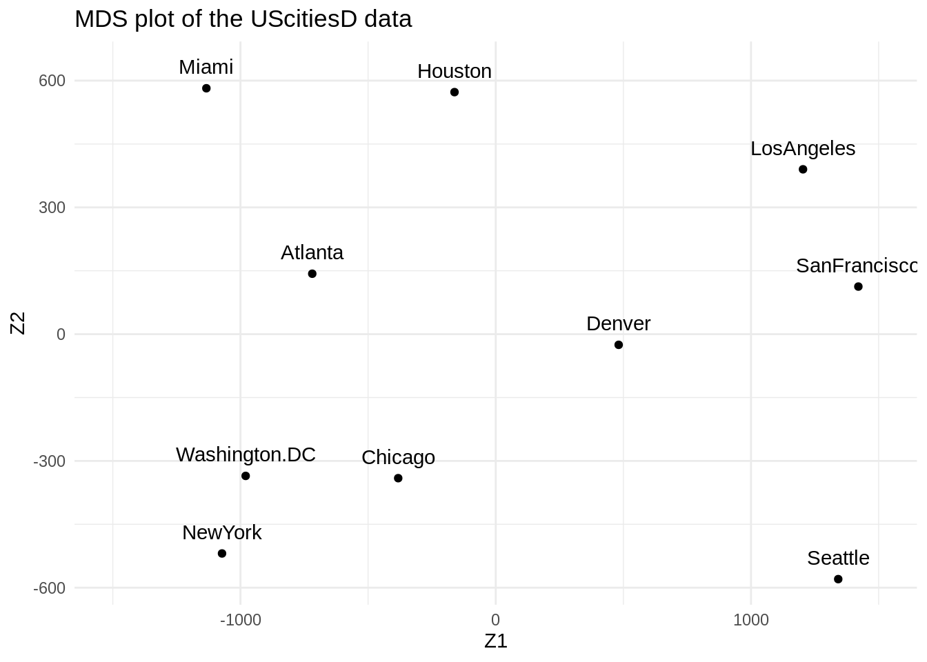

What can you say about the plot? Think about the real locations of these cities on a map of the US.

Answer

\(Z_1\) can be interpreted as the longitude, i.e. the East-West position. \(Z_2\) reflects the latitude, or the North-South position.

2.2 The short way

The calculations above demonstrate how MDS works and what the underlying components are. However, in a real data analysis, one would typically not go through all the hassle of calculating all the intermediate steps. Fortunately, the MDS is already implemented in base R (in the stats package).

So the whole derivation we did above can be reproduced with a single line of code, using the cmdscale function (see ?cmdscale for details).

## Calculate MDS in 2 dimensions from distance matrix
(us_mds <- cmdscale(UScitiesD, k = 2))
#>                     [,1]       [,2]
#> Atlanta        -718.7594  142.99427
#> Chicago        -382.0558 -340.83962
#> Denver          481.6023  -25.28504
#> Houston        -161.4663  572.76991
#> LosAngeles     1203.7380  390.10029
#> Miami         -1133.5271  581.90731
#> NewYork       -1072.2357 -519.02423
#> SanFrancisco   1420.6033  112.58920
#> Seattle        1341.7225 -579.73928
#> Washington.DC  -979.6220 -335.47281
colnames(us_mds) <- c("Z1", "Z2")

## Plot MDS
us_mds %>%
  as_tibble(rownames = "city") %>%
  ggplot(aes(Z1, Z2, label = city)) +
  geom_point() +
  geom_text(nudge_y = 50) +
  xlim(c(-1500, 1500)) +
  theme_minimal()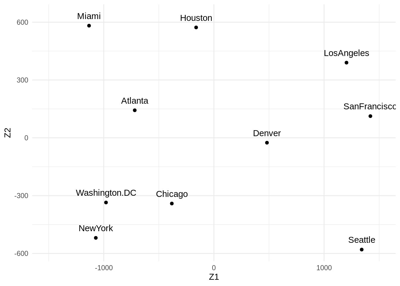

Which gives us the same result as before (which is a good check that we didn’t make mistakes!).

3 Exercises

3.1 Cheese data

Data prep

Load in the cheese data, which characterizes 30 cheeses on various metrics. More information can be found at ?cheese

## Load the 'cheese' dataset from the HDDAData package
data("cheese")
cheese

Q: what is the dimensionality of this data?

Answer

A: 4, since we have 4 features (the first column is just an identifier for the observation, so we don’t regard this as a feature).

ncol(cheese) - 1
#> [1] 4

Convert the cheese table to a matrix for easier calculations. We will drop the first column (as it’s not a feature) and instead use it to create rownames.

cheese_mx <- as.matrix(cheese[, -1])
rownames(cheese_mx) <- paste("case", cheese$Case, sep = "_")
cheese_mx
#>         taste Acetic    H2S Lactic
#> case_1   12.3  4.543  3.135   0.86
#> case_2   20.9  5.159  5.043   1.53
#> case_3   39.0  5.366  5.438   1.57
#> case_4   47.9  5.759  7.496   1.81
#> case_5    5.6  4.663  3.807   0.99
#> case_6   25.9  5.697  7.601   1.09
#> case_7   37.3  5.892  8.726   1.29
#> case_8   21.9  6.078  7.966   1.78
#> case_9   18.1  4.898  3.850   1.29
#> case_10  21.0  5.242  4.174   1.58
#> case_11  34.9  5.740  6.142   1.68
#> case_12  57.2  6.446  7.908   1.90
#> case_13   0.7  4.477  2.996   1.06
#> case_14  25.9  5.236  4.942   1.30
#> case_15  54.9  6.151  6.752   1.52
#> case_16  40.9  6.365  9.588   1.74
#> case_17  15.9  4.787  3.912   1.16
#> case_18   6.4  5.412  4.700   1.49
#> case_19  18.0  5.247  6.174   1.63
#> case_20  38.9  5.438  9.064   1.99
#> case_21  14.0  4.564  4.949   1.15
#> case_22  15.2  5.298  5.220   1.33
#> case_23  32.0  5.455  9.242   1.44
#> case_24  56.7  5.855 10.199   2.01
#> case_25  16.8  5.366  3.664   1.31
#> case_26  11.6  6.043  3.219   1.46
#> case_27  26.5  6.458  6.962   1.72
#> case_28   0.7  5.328  3.912   1.25
#> case_29  13.4  5.802  6.685   1.08
#> case_30   5.5  6.176  4.787   1.25

Check rank of cheese_mx and center the matrix.

qr(cheese_mx)$rank
#> [1] 4

# Centering the data matrix
n <- nrow(cheese_mx)
cheese_H <- diag(n) - 1 / n * matrix(1, ncol = n, nrow = n)
cheese_centered <- cheese_H %*% as.matrix(cheese_mx)
## Again we use H here because we use it for some exercises later on
## In real-life applications using the `scale` function would be more appropriate

Tasks

Note: no need for mathematical derivations, just verify code-wise in R.

We obtained the column-centered data matrix \(\mathbf{X}\) after multiplying the original matrix with

\[ \mathbf{H} = \mathbf{I} - \frac{1}{n} \mathbf{1}\mathbf{1}^T \]

1. Show that \(\mathbf{X}\) (here: cheese_centered) is indeed column-centered (and not row-centered)

Solution

# X is indeed column-centered:
round(colMeans(cheese_centered), 14) ## practically zero
#>  taste Acetic    H2S Lactic 
#>      0      0      0      0

# but it is not row-centered:
 rowMeans(cheese_centered)
#>  [1] -4.144283333 -1.195783333  3.489716667  6.387466667 -5.588783333
#>  [6]  0.718216667  3.948216667  0.077216667 -2.319283333 -1.354783333
#> [11]  2.761716667  9.009716667 -7.045533333 -0.009283333  7.976966667
#> [16]  5.294466667 -2.914033333 -4.853283333 -1.591033333  4.494216667
#> [21] -3.188033333 -2.591783333  2.680466667  9.337216667 -2.568783333
#> [26] -3.773283333  1.056216667 -6.556283333 -2.612033333 -4.925533333

2. Verify that whenever \(\mathbf{X}\) is column-centered, the equality \(\mathbf{HX = X}\) holds

Solution

# verifying that HX = X
all.equal(cheese_H %*% cheese_centered, cheese_centered)
#> [1] TRUE

3. Perform an SVD on cheese_centered, and store the matrices \(\mathbf{U}\), \(\mathbf{V}\) and \(\mathbf{\Delta}\) as separate objects

Solution

cheese_svd <- svd(cheese_centered)
str(cheese_svd)
#> List of 3
#>  $ d: num [1:4] 87.99 7.53 2.39 1.06
#>  $ u: num [1:30, 1:4] -0.1418 -0.0422 0.163 0.266 -0.2167 ...
#>  $ v: num [1:4, 1:4] 0.9948 0.0193 0.0991 0.0131 0.1013 ...
U <- cheese_svd$u
V <- cheese_svd$v
D <- diag(cheese_svd$d)

4. Show that \(\mathbf{u_1}\) is a normalized vector; show the same for \(\mathbf{u_2}\). Show that \(\mathbf{u_1}\) and \(\mathbf{u_2}\) are orthogonal vectors. Then show the orthonormality of all vectors \(\mathbf{u_j}\) in a single calculation (using the matrix \(\mathbf{U}\)). Similarly, show the orthonormality of all vectors \(\mathbf{v_j}\) in a single calculation (using the matrix \(\mathbf{V}\)).

Solution

# Verifying orthonormality
# ------------------------
# The vectors u1 and u2 are orthonormal
t(U[, 1]) %*% U[, 1]
#>      [,1]
#> [1,]    1
t(U[, 2]) %*% U[, 2]
#>      [,1]
#> [1,]    1
t(U[, 1]) %*% U[, 2]
#>              [,1]
#> [1,] 2.775558e-17

# Verifying that U forms an orthonormal basis in one step:
t(U) %*% U # computational imperfections
#>               [,1]          [,2]          [,3]         [,4]
#> [1,]  1.000000e+00  2.775558e-17 -1.942890e-16 3.469447e-17
#> [2,]  2.775558e-17  1.000000e+00 -2.081668e-17 6.938894e-18
#> [3,] -1.942890e-16 -2.081668e-17  1.000000e+00 8.326673e-17
#> [4,]  3.469447e-17  6.938894e-18  8.326673e-17 1.000000e+00
round(t(U) %*% U, digits = 15)
#>      [,1] [,2] [,3] [,4]
#> [1,]    1    0    0    0
#> [2,]    0    1    0    0
#> [3,]    0    0    1    0
#> [4,]    0    0    0    1


# Verifying that V forms an orthonormal basis:
t(V) %*% V # computational imperfections
#>              [,1]          [,2]          [,3]          [,4]
#> [1,] 1.000000e+00  2.168404e-19  9.107298e-18  1.734723e-18
#> [2,] 2.168404e-19  1.000000e+00  1.162265e-16 -4.163336e-17
#> [3,] 9.107298e-18  1.162265e-16  1.000000e+00 -1.387779e-16
#> [4,] 1.734723e-18 -4.163336e-17 -1.387779e-16  1.000000e+00
round(t(V) %*% V, digits = 15)
#>      [,1] [,2] [,3] [,4]
#> [1,]    1    0    0    0
#> [2,]    0    1    0    0
#> [3,]    0    0    1    0
#> [4,]    0    0    0    1

5. Check that the SVD was performed correctly, i.e. calculate the matrix \(\mathbf{X}\) from the elements of the SVD.

Solution

There are 2 ways to do this

• Using the sum definition of the SVD \(\mathbf{X} = \sum_{j=1}^r \delta_j \mathbf{u}_j\mathbf{v}_j^T\)

# Calculating X via the sum definition of the SVD:
# ------------------------------------------------

## Initialize empty matrix
X_sum <- matrix(0, nrow = nrow(U), ncol = ncol(V))

## Compute sum by looping over columns
for (j in 1:ncol(U)) {
  X_sum <- X_sum + (diag(D)[j] * U[, j] %*% t(V[, j]))
}

• using the matrix notation of the SVD

\(\mathbf{X}=\mathbf{U}_{n\times n}\boldsymbol{\Delta}_{n\times p}\mathbf{V}^T_{p \times p}\)

# Calculating X via the SVD matrix multiplication:
# ------------------------------------------------
X_mult <- U %*% D %*% t(V)

• Verify that the obtained results are identical to the matrix \(\mathbf{X}\).

## Remove dimnames with unname for comparison
all.equal(X_sum, unname(cheese_centered))
#> [1] TRUE
all.equal(X_mult, unname(cheese_centered))
#> [1] TRUE

6. Approximate the matrix \(\mathbf{\tilde{\mathbf{X}}}\), for \(k = 2\) using the truncated SVD.

Solution

Using the matrix notation of the SVD \(\tilde{\mathbf{X}}=\mathbf{U}_{n\times k}\boldsymbol{\Delta}_{k\times k}\mathbf{V}_{p \times k}^T\)

k <- 2
X_tilde <- U[, 1:k] %*% D[1:k,1:k] %*% t(V[,1:k])
X_tilde
#>             [,1]         [,2]       [,3]        [,4]
#>  [1,] -12.239133 -0.473616046 -2.8890844 -0.22869032
#>  [2,]  -3.632893 -0.149296787 -0.9192007 -0.07036869
#>  [3,]  14.466098  0.003193815 -0.5222165  0.11143994
#>  [4,]  23.367068  0.343030388  1.5463259  0.27644233
#>  [5,] -18.937322 -0.412170627 -2.2022031 -0.26233046
#>  [6,]   1.362512  0.238584208  1.6362609  0.07850579
#>  [7,]  12.762842  0.458129158  2.7598179  0.22827153
#>  [8,]  -2.629186  0.279768668  2.0779016  0.05976183
#>  [9,]  -6.434808 -0.335320743 -2.1294786 -0.14487077
#> [10,]  -3.531065 -0.267124541 -1.7564651 -0.10322047
#> [11,]  10.368716  0.087369057  0.2274905  0.10415872
#> [12,]  32.669955  0.462076014  2.0380140  0.38149853
#> [13,] -23.836211 -0.552972271 -3.0136366 -0.33994737
#> [14,]   1.364965 -0.137217299 -1.0219832 -0.02873484
#> [15,]  30.366491  0.282301907  0.8531709  0.31258868
#> [16,]  16.368042  0.607820015  3.6828489  0.29854111
#> [17,]  -8.636391 -0.341018561 -2.0868672 -0.16331822
#> [18,] -18.129963 -0.266973043 -1.2055849 -0.21472027
#> [19,]  -6.532447 -0.005490492  0.2071824 -0.05147830
#> [20,]  14.366327  0.508218560  3.0537258  0.25481924
#> [21,] -10.538563 -0.211763797 -1.1009736 -0.14096055
#> [22,]  -9.333559 -0.152667016 -0.7283467 -0.11488660
#> [23,]   7.461972  0.494423480  3.2161739  0.19812912
#> [24,]  32.165441  0.765561370  4.2036533  0.46426305
#> [25,]  -7.731858 -0.358497140 -2.2445637 -0.16139578
#> [26,] -12.925926 -0.432844491 -2.5748303 -0.22230096
#> [27,]   1.972823  0.171717046  1.1403054  0.06408399
#> [28,] -23.831087 -0.408474088 -1.9917525 -0.29866628
#> [29,] -11.134642  0.049222629  0.7675071 -0.07102548
#> [30,] -19.028198 -0.245969372 -1.0231915 -0.21558848

• Compare the obtained results with the matrix \(\mathbf{X}\) (cheese_centered). Just at a first glance, does it seem that \(\mathbf{\tilde{X}}\) is a good approximation of \(\mathbf{X}\)?

7. SVD and linear regression: perform a linear regression using SVD to estimate the effects of the Acetic, H2S and Lactic variables on the taste.

Note: we cannot use the SVD from before as this was calculated from the complete cheese table, also including the taste column, which is the response variable of interest here. Instead, we need to create a new design matrix \(\mathbf{X}\) containing the predictors and a separate vector \(\mathbf{y}\) containing the response.

cheese_y <- cheese$taste
cheese_design <- cbind(Intercept = 1, cheese[c("Acetic", "H2S", "Lactic")])

Also perform the regression with lm and compare the results.

Solution

## Fit with lm
lm_fit <- lm(taste ~ Acetic + H2S + Lactic, data = cheese)

## Fit with SVD
design_svd <- svd(cheese_design)
svd_coef <- design_svd$v %*% diag(1/design_svd$d) %*% t(design_svd$u) %*% cheese_y

## Compare
cbind(
  "lm" = coef(lm_fit),
  "svd" = drop(svd_coef)
)
#>                      lm         svd
#> (Intercept) -28.8767696 -28.8767696
#> Acetic        0.3277413   0.3277413
#> H2S           3.9118411   3.9118411
#> Lactic       19.6705434  19.6705434

3.2 Exercise: employment by industry in European countries

In this exercise we will focus on the interpretation of the biplot.

Data prep

The "industries" dataset contains data on the distribution of employment between 9 industrial sectors, in 26 European countries. The dataset stems from the Cold-War era; the data are expressed as percentages. Load the data and explore its contents.

## Load 'industries' data from the HDDAData package
data("industries")

# Explore contents
industries

dim(industries)
#> [1] 26 10
summary(industries)
#>    country           agriculture        mining      manufacturing  
#>  Length:26          Min.   : 2.70   Min.   :0.100   Min.   : 7.90  
#>  Class :character   1st Qu.: 7.70   1st Qu.:0.525   1st Qu.:23.00  
#>  Mode  :character   Median :14.45   Median :0.950   Median :27.55  
#>                     Mean   :19.13   Mean   :1.254   Mean   :27.01  
#>                     3rd Qu.:23.68   3rd Qu.:1.800   3rd Qu.:30.20  
#>                     Max.   :66.80   Max.   :3.100   Max.   :41.20  
#>   power.supply     construction       services        finance      
#>  Min.   :0.1000   Min.   : 2.800   Min.   : 5.20   Min.   : 0.500  
#>  1st Qu.:0.6000   1st Qu.: 7.525   1st Qu.: 9.25   1st Qu.: 1.225  
#>  Median :0.8500   Median : 8.350   Median :14.40   Median : 4.650  
#>  Mean   :0.9077   Mean   : 8.165   Mean   :12.96   Mean   : 4.000  
#>  3rd Qu.:1.1750   3rd Qu.: 8.975   3rd Qu.:16.88   3rd Qu.: 5.925  
#>  Max.   :1.9000   Max.   :11.500   Max.   :19.10   Max.   :11.300  
#>  social.sector     transport    
#>  Min.   : 5.30   Min.   :3.200  
#>  1st Qu.:16.25   1st Qu.:5.700  
#>  Median :19.65   Median :6.700  
#>  Mean   :20.02   Mean   :6.546  
#>  3rd Qu.:24.12   3rd Qu.:7.075  
#>  Max.   :32.40   Max.   :9.400

Create data matrix \(\mathbf{X}\).

# Create matrix without first column ("country", which will be used for rownames)
indus_X <- as.matrix(industries[, -1])
rownames(indus_X) <- industries$country

# Check the dimensionality
dim(indus_X)
#> [1] 26  9

# and the rank
qr(indus_X)$rank
#> [1] 9

# n will be used subsequently
n <- nrow(indus_X)

Tasks

1. Perform a truncated SVD for \(k=2\), and construct the biplot accordingly.

Solution

# Centering the data matrix first
# H <- diag(n) - 1 / n * matrix(1, ncol = n, nrow = n)
# indus_centered <- H %*% as.matrix(indus_X)
indus_centered <- scale(indus_X, scale = FALSE)

# Perform SVD
indus_svd <- svd(indus_centered)
str(indus_svd)
#> List of 3
#>  $ d: num [1:9] 87.1 33.05 19.5 11.87 7.82 ...
#>  $ u: num [1:26, 1:9] -0.2011 -0.132 -0.1048 -0.1653 0.0512 ...
#>  $ v: num [1:9, 1:9] 0.89176 0.00192 -0.27127 -0.00839 -0.04959 ...

# Extract singular vectors for k = 2 and calculate k=2 projection Zk
k <- 2
Uk <- indus_svd$u[ , 1:k]
Dk <- diag(indus_svd$d[1:k])

Vk <- indus_svd$v[, 1:k]
rownames(Vk) <- colnames(indus_X)
colnames(Vk) <- c("V1", "V2")

Zk <- Uk %*% Dk
rownames(Zk) <- industries$country
colnames(Zk) <- c("Z1", "Z2")
Zk
#>                        Z1           Z2
#> Belgium        -17.516687  -4.92622849
#> Denmark        -11.496688 -11.66176637
#> France          -9.128686  -2.16828207
#> W. Germany     -14.393424   5.04749385
#> Ireland          4.458174  -6.13156498
#> Italy           -4.026684  -0.38889529
#> Luxembourg     -12.089752   2.33236877
#> Netherlands    -13.900455  -9.72359023
#> UK             -18.728675  -3.33178946
#> Austria         -6.471418   3.35662962
#> Finland         -6.837047  -3.97634061
#> Greece          25.427083  -1.80467718
#> Norway         -10.972019  -8.85877780
#> Portugal         9.403865  -0.08570061
#> Spain            5.774973   6.15867547
#> Sweden         -15.311975  -8.52674423
#> Switzerland    -12.683839   9.77920054
#> Turkey          52.115644  -8.64165980
#> Bulgaria         4.156791   6.70685051
#> Czechoslovakia  -3.246127   9.23467980
#> E. Germany     -17.415527  10.73233092
#> Hungary          3.135737   4.98695108
#> Poland          13.315709   2.94482700
#> Romania         17.011336   9.12523022
#> USSR             4.587043  -0.87197041
#> Yugoslavia      34.832648   0.69274975

Biplot with ggplot2:

## Scale factor to draw Vk arrows (can be set arbitrarily)
scale_factor <- 20

## Create tibble with rownames in "country" column
as_tibble(Zk, rownames = "country") %>%
  ggplot(aes(Z1, Z2)) +
  geom_point() +
  geom_text(aes(label = country), size = 3, nudge_y = 0.5) +
  ## Plot Singular vectors Vk
  geom_segment(
    data = as_tibble(Vk, rownames = "sector"),
    aes(x = 0, y = 0, xend = V1 * scale_factor, yend = V2 * scale_factor),
    arrow = arrow(length = unit(0.4, "cm")),
    color = "firebrick"
  ) +
  geom_text(
    data = as_tibble(Vk, rownames = "sector"),
    aes(V1 * scale_factor, V2 * scale_factor, label = sector),
    nudge_x = 0.5, nudge_y = ifelse(Vk[, 2] >= 0, 0.5, -0.5),
    color = "firebrick", size = 3
  ) +
  theme_minimal()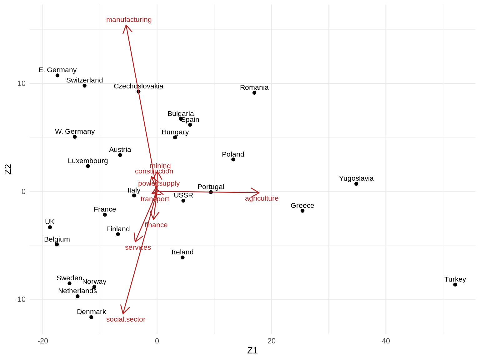

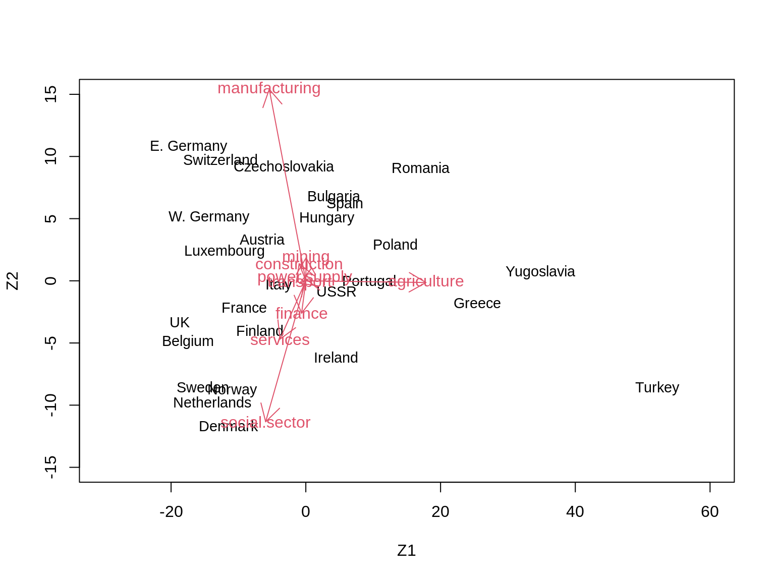
Using base R:

# # Constructing the biplot for Z1 and Z2
#  # -------------------------------------
plot(Zk[, 1:2],
  type = "n", xlim = c(-30, 60), ylim = c(-15, 15),
  xlab = "Z1", ylab = "Z2"
)
text(Zk[, 1:2], rownames(Zk), cex = 0.9)
# alpha <- 1
alpha <- 20 # rescaling to get better visualisation
for (i in 1:9) {
  arrows(0, 0, alpha * Vk[i, 1], alpha * Vk[i, 2], length = 0.2, col = 2)
  text(alpha * Vk[i, 1], alpha * Vk[i, 2], rownames(Vk)[i], col = 2)
}

2. To see if we can learn more when retaining more dimensions, repeat the truncated SVD for \(k=3\). Construct two-dimensional biplots for:

• Z1 and Z3
• Z2 and Z3

Solution

No need to re-do SVD, just extract singular vectors for \(k=3\) from previous SVD.

# Extract singular vectors for k = 3 and calculate projection Zk
k <- 3
Uk <- indus_svd$u[ , 1:k]
Dk <- diag(indus_svd$d[1:k])

Vk <- indus_svd$v[, 1:k]
rownames(Vk) <- colnames(indus_X)
colnames(Vk) <- c("V1", "V2", "V3")

Zk <- Uk %*% Dk
rownames(Zk) <- industries$country
colnames(Zk) <- c("Z1", "Z2", "Z3")
Zk
#>                        Z1           Z2          Z3
#> Belgium        -17.516687  -4.92622849 -2.35528094
#> Denmark        -11.496688 -11.66176637  3.00202830
#> France          -9.128686  -2.16828207 -2.75030568
#> W. Germany     -14.393424   5.04749385  0.20568951
#> Ireland          4.458174  -6.13156498 -1.92400082
#> Italy           -4.026684  -0.38889529 -2.40586194
#> Luxembourg     -12.089752   2.33236877 -4.62806669
#> Netherlands    -13.900455  -9.72359023 -1.70981367
#> UK             -18.728675  -3.33178946  0.58938403
#> Austria         -6.471418   3.35662962 -4.75660272
#> Finland         -6.837047  -3.97634061  0.06757235
#> Greece          25.427083  -1.80467718 -2.91613130
#> Norway         -10.972019  -8.85877780  0.22621023
#> Portugal         9.403865  -0.08570061 -1.23656256
#> Spain            5.774973   6.15867547 -4.87904446
#> Sweden         -15.311975  -8.52674423  3.92210148
#> Switzerland    -12.683839   9.77920054 -5.68921238
#> Turkey          52.115644  -8.64165980  2.96515501
#> Bulgaria         4.156791   6.70685051  4.93995679
#> Czechoslovakia  -3.246127   9.23467980  3.78225558
#> E. Germany     -17.415527  10.73233092  4.89564722
#> Hungary          3.135737   4.98695108  2.98354179
#> Poland          13.315709   2.94482700  3.58894681
#> Romania         17.011336   9.12523022  2.58152423
#> USSR             4.587043  -0.87197041  8.44875566
#> Yugoslavia      34.832648   0.69274975 -6.94788580

Create biplot as before.

• Z1 vs. Z3

## Scale factor to draw Vk arrows (can be set arbitrarily)
scale_factor <- 20

## Create tibble with rownames in "country" column
as_tibble(Zk, rownames = "country") %>%
  ggplot(aes(Z1, Z3)) +
  geom_point() +
  geom_text(aes(label = country), size = 3, nudge_y = 0.5) +
  ## Plot Singular vectors Vk
  geom_segment(
    data = as_tibble(Vk, rownames = "sector"),
    aes(x = 0, y = 0, xend = V1 * scale_factor, yend = V3 * scale_factor),
    arrow = arrow(length = unit(0.4, "cm")),
    color = "firebrick"
  ) +
  geom_text(
    data = as_tibble(Vk, rownames = "sector"),
    aes(V1 * scale_factor, V3 * scale_factor, label = sector),
    nudge_x = 0.5, nudge_y = ifelse(Vk[, 3] >= 0, 0.5, -0.5),
    color = "firebrick", size = 3
  ) +
  theme_minimal()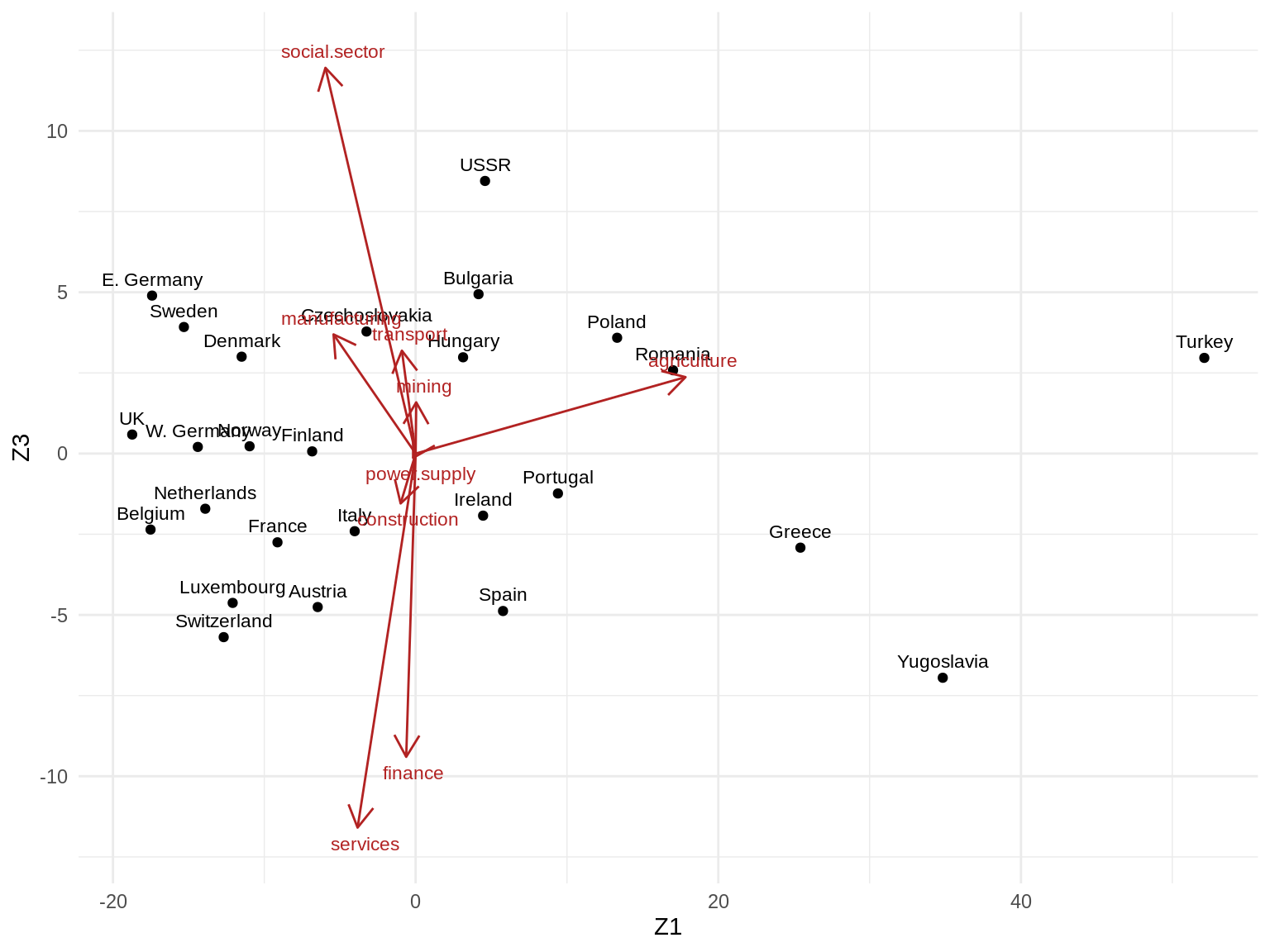

• Z2 vs. Z3

# Scale factor to draw Vk arrows (can be set arbitrarily)
scale_factor <- 20

## Create tibble with rownames in "country" column
as_tibble(Zk, rownames = "country") %>%
  ggplot(aes(Z2, Z3)) +
  geom_point() +
  geom_text(aes(label = country), size = 3, nudge_y = 0.5) +
  ## Plot Singular vectors Vk
  geom_segment(
    data = as_tibble(Vk, rownames = "sector"),
    aes(x = 0, y = 0, xend = V2 * scale_factor, yend = V3 * scale_factor),
    arrow = arrow(length = unit(0.4, "cm")),
    color = "firebrick"
  ) +
  geom_text(
    data = as_tibble(Vk, rownames = "sector"),
    aes(V2 * scale_factor, V3 * scale_factor, label = sector),
    nudge_x = 0.5, nudge_y = ifelse(Vk[, 3] >= 0, 0.5, -0.5),
    color = "firebrick", size = 3
  ) +
  theme_minimal()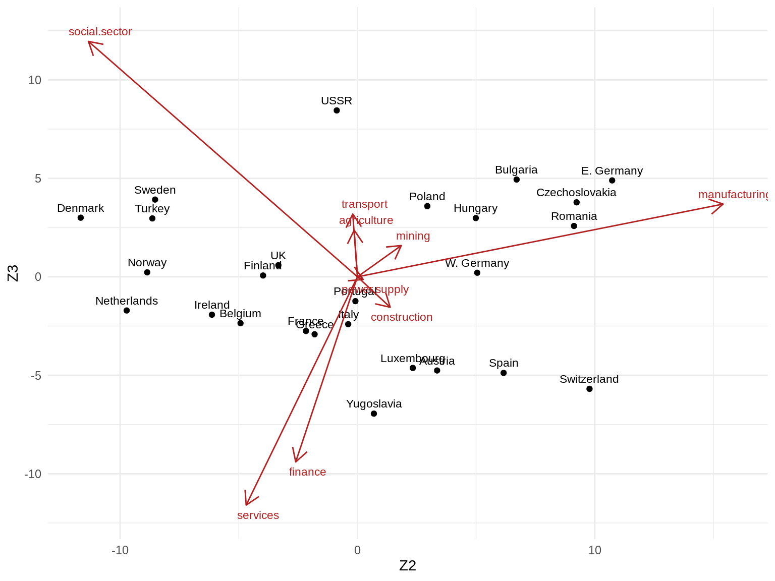

3. Can you give a meaningful interpretation to each dimension?

Session info

Session info

#> [1] "2022-01-25 11:17:02 UTC"
#> ─ Session info ───────────────────────────────────────────────────────────────
#>  setting  value
#>  version  R version 4.1.2 (2021-11-01)
#>  os       Ubuntu 20.04.3 LTS
#>  system   x86_64, linux-gnu
#>  ui       X11
#>  language (EN)
#>  collate  C.UTF-8
#>  ctype    C.UTF-8
#>  tz       UTC
#>  date     2022-01-25
#>  pandoc   2.7.3 @ /usr/bin/ (via rmarkdown)
#> 
#> ─ Packages ───────────────────────────────────────────────────────────────────
#>  ! package     * version date (UTC) lib source
#>  P assertthat    0.2.1   2019-03-21 [?] CRAN (R 4.1.2)
#>  P backports     1.2.1   2020-12-09 [?] CRAN (R 4.1.2)
#>  P BiocManager   1.30.16 2021-06-15 [?] CRAN (R 4.1.2)
#>  P broom         0.7.9   2021-07-27 [?] CRAN (R 4.1.2)
#>  P bslib         0.3.0   2021-09-02 [?] CRAN (R 4.1.2)
#>  P cellranger    1.1.0   2016-07-27 [?] CRAN (R 4.1.2)
#>  P cli           3.1.1   2022-01-20 [?] CRAN (R 4.1.2)
#>  P colorspace    2.0-2   2021-06-24 [?] CRAN (R 4.1.2)
#>  P crayon        1.4.1   2021-02-08 [?] CRAN (R 4.1.2)
#>  P DBI           1.1.1   2021-01-15 [?] CRAN (R 4.1.2)
#>  P dbplyr        2.1.1   2021-04-06 [?] CRAN (R 4.1.2)
#>  P digest        0.6.28  2021-09-23 [?] CRAN (R 4.1.2)
#>  P dplyr       * 1.0.7   2021-06-18 [?] CRAN (R 4.1.2)
#>  P ellipsis      0.3.2   2021-04-29 [?] CRAN (R 4.1.2)
#>  P evaluate      0.14    2019-05-28 [?] CRAN (R 4.1.2)
#>  P fansi         0.5.0   2021-05-25 [?] CRAN (R 4.1.2)
#>  P farver        2.1.0   2021-02-28 [?] CRAN (R 4.1.2)
#>  P fastmap       1.1.0   2021-01-25 [?] CRAN (R 4.1.2)
#>  P forcats     * 0.5.1   2021-01-27 [?] CRAN (R 4.1.2)
#>  P fs            1.5.0   2020-07-31 [?] CRAN (R 4.1.2)
#>  P generics      0.1.0   2020-10-31 [?] CRAN (R 4.1.2)
#>  P ggplot2     * 3.3.5   2021-06-25 [?] CRAN (R 4.1.2)
#>  P glue          1.4.2   2020-08-27 [?] CRAN (R 4.1.2)
#>  P gtable        0.3.0   2019-03-25 [?] CRAN (R 4.1.2)
#>  P haven         2.4.3   2021-08-04 [?] CRAN (R 4.1.2)
#>  P HDDAData    * 0.0.2   2022-01-25 [?] Github (statOmics/HDDAData@d6ab354)
#>  P highr         0.9     2021-04-16 [?] CRAN (R 4.1.2)
#>  P hms           1.1.1   2021-09-26 [?] CRAN (R 4.1.2)
#>  P htmltools     0.5.2   2021-08-25 [?] CRAN (R 4.1.2)
#>  P httr          1.4.2   2020-07-20 [?] CRAN (R 4.1.2)
#>  P jquerylib     0.1.4   2021-04-26 [?] CRAN (R 4.1.2)
#>  P jsonlite      1.7.2   2020-12-09 [?] CRAN (R 4.1.2)
#>  P knitr         1.33    2021-04-24 [?] CRAN (R 4.1.2)
#>  P labeling      0.4.2   2020-10-20 [?] CRAN (R 4.1.2)
#>  P lifecycle     1.0.1   2021-09-24 [?] CRAN (R 4.1.2)
#>  P lubridate     1.7.10  2021-02-26 [?] CRAN (R 4.1.2)
#>  P magrittr      2.0.1   2020-11-17 [?] CRAN (R 4.1.2)
#>  P modelr        0.1.8   2020-05-19 [?] CRAN (R 4.1.2)
#>  P munsell       0.5.0   2018-06-12 [?] CRAN (R 4.1.2)
#>  P pillar        1.6.3   2021-09-26 [?] CRAN (R 4.1.2)
#>  P pkgconfig     2.0.3   2022-01-25 [?] Github (r-lib/pkgconfig@b81ae03)
#>  P purrr       * 0.3.4   2020-04-17 [?] CRAN (R 4.1.2)
#>  P R6            2.5.1   2021-08-19 [?] CRAN (R 4.1.2)
#>  P Rcpp          1.0.7   2021-07-07 [?] CRAN (R 4.1.2)
#>  P readr       * 2.0.1   2021-08-10 [?] CRAN (R 4.1.2)
#>  P readxl        1.3.1   2019-03-13 [?] CRAN (R 4.1.2)
#>  P renv          0.15.2  2022-01-24 [?] CRAN (R 4.1.2)
#>  P reprex        2.0.1   2021-08-05 [?] CRAN (R 4.1.2)
#>  P rlang         0.4.11  2021-04-30 [?] CRAN (R 4.1.2)
#>  P rmarkdown     2.10    2021-08-06 [?] CRAN (R 4.1.2)
#>  P rstudioapi    0.13    2020-11-12 [?] CRAN (R 4.1.2)
#>  P rvest         1.0.1   2021-07-26 [?] CRAN (R 4.1.2)
#>  P sass          0.4.0   2021-05-12 [?] CRAN (R 4.1.2)
#>  P scales        1.1.1   2020-05-11 [?] CRAN (R 4.1.2)
#>  P sessioninfo   1.2.2   2021-12-06 [?] CRAN (R 4.1.2)
#>  P stringi       1.7.4   2021-08-25 [?] CRAN (R 4.1.2)
#>  P stringr     * 1.4.0   2019-02-10 [?] CRAN (R 4.1.2)
#>  P tibble      * 3.1.5   2021-09-30 [?] CRAN (R 4.1.2)
#>  P tidyr       * 1.1.4   2021-09-27 [?] CRAN (R 4.1.2)
#>  P tidyselect    1.1.1   2021-04-30 [?] CRAN (R 4.1.2)
#>  P tidyverse   * 1.3.1   2021-04-15 [?] CRAN (R 4.1.2)
#>  P tzdb          0.1.2   2021-07-20 [?] CRAN (R 4.1.2)
#>  P utf8          1.2.2   2021-07-24 [?] CRAN (R 4.1.2)
#>  P vctrs         0.3.8   2021-04-29 [?] CRAN (R 4.1.2)
#>  P withr         2.4.2   2021-04-18 [?] CRAN (R 4.1.2)
#>  P xfun          0.25    2021-08-06 [?] CRAN (R 4.1.2)
#>  P xml2          1.3.2   2020-04-23 [?] CRAN (R 4.1.2)
#>  P yaml          2.2.1   2020-02-01 [?] CRAN (R 4.1.2)
#> 
#>  [1] /home/runner/work/HDDA21/HDDA21/renv/library/R-4.1/x86_64-pc-linux-gnu
#>  [2] /opt/R/4.1.2/lib/R/library
#> 
#>  P ── Loaded and on-disk path mismatch.
#> 
#> ──────────────────────────────────────────────────────────────────────────────

---

This work is licensed under the CC BY-NC-SA 4.0 licence.