---
title: "Tutorial: Intro to DIA proteomics data processing"
code-tools: true
author:
- name: Lieven Clement
orcid: 0000-0002-9050-4370
affiliation:
- name: Ghent University
---
# Background
We will use using a publicly available spike-in study published by Staes et al. [@Staes2024].
They spiked digested UPS proteins in a yeast digested background at the following ratio's (yeast:ups ratio 10:1, 10:2, 10:4, 10:8, 10:10).
Here we will use a subset of the data, i.e. dilutions 10:2 and 10:4.
We will use output of the search engine DIA-NN 2.2.0.
The main search output for this DIA-NN version was stored in the report.parquet file in the DIA-NN output directory, which can be found under data/spikein24-staesetal2024.parquet
DIA-NN provides multiple quantifications, e.g. derived from the MS1 or MS2 spectra, and at precursor or protein (protein group) level. The term 'precursor' refers to a charged peptide species and is the basic unit of identification and quantification in DIA. Hence, in the context of DIA we refer to a precursor table, instead of to a PSM table in DDA.
Examples of different quantities are:
- raw MS1 area: Ms1.Area, normalised MS1 Area: Ms1.Normalised, MS2 Precursor quantities: Precursor.Quantity, Normalised MS2 Precursor quantities: Precursor.Normalised, etc., which are all at the precursor level
- MS2 based summary at the protein (protein group)-level: PG.MaxLFQ
Here, we will use the `Precursor.Quantity` column.
# Load packages
We load the `msqrob2` package, along with additional packages for
data manipulation and visualisation.
```{r load_libraries}
library("QFeatures")
library("dplyr")
library("tidyr")
library("ggplot2")
library("msqrob2")
library("stringr")
library("ExploreModelMatrix")
library("MsCoreUtils")
library("matrixStats")
library("patchwork")
library("kableExtra")
library("ComplexHeatmap")
library("purrr")
library("tibble")
library("scater")
```
# Data
## Precursor table
We load the output from DIA-NN parquet file. Can be file path to local file or url to file that lives on the web.
```{r import_data}
precursorFile <- "https://github.com/statOmics/msqrob2data/raw/refs/heads/main/dia/spikeinStaes/spikein24-staesetal2024.parquet"
```
We can import the report.parquet file using the `read_parquet` function from the `arrow` package.
Note, that older versions of DIA-NN store the output as report.tsv.
```{r}
precursors <- arrow::read_parquet(precursorFile) # function from the arrow package
#precursors <- data.table::fread(precursorFile) # For older versions of DIA-NN, where the results are stored as tsv files. Note that the precursorFile then would point to "report.tsv"
```
Each row in the precursor data table is in "long format" and contains information about one precursor in a specific run (the table below shows the first 6 rows).
The columns contains various descriptors about the precursor, such as its sequence, its charge, run, etc. Some of these columns contain the quantification values, e.g. Ms1.Area, Precursor.Quantity etc.
```{r, echo=FALSE}
knitr::kable(head(precursors))
```
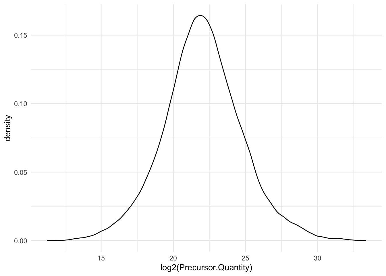
Quick check on distribution of precursors MS2 intensities.
```{r}
precursors |>
  ggplot(aes(x = log2(Precursor.Quantity))) +
  geom_density() +
  theme_minimal()
```
We filter the data to reduce the memory footprint.
```{r}
precursors <- precursors |>
  select(
         Run,
         Precursor.Id,
         Modified.Sequence,
         Stripped.Sequence,
         Precursor.Charge,
         Protein.Group,
         Protein.Names,
         Protein.Ids,
         Genes,
         Precursor.Quantity,
         Precursor.Normalised,
         Normalisation.Factor,
         Ms1.Area,
         Ms1.Normalised,
         PG.MaxLFQ,
         Q.Value,
         Lib.Q.Value,
         PG.Q.Value,
         Lib.PG.Q.Value,
         Proteotypic,
         Decoy, # Not available in older versions of DIA-NN
         RT)
```
We known the ground truth: UPS proteins are differentially abundant (DA, spiked in), Yeast proteins are not.
```{r}
precursors <- precursors |>
  mutate(species = grepl(pattern = "UPS",Protein.Group) |>
           as.factor() |>
           recode("TRUE"="ups","FALSE" = "yeast"))
precursors |>
  pull(species) |>
  table()
```
## Sample annotation table
The [sample annotation table](#sec-annotation_table)) is not available
and can be generated from the run labels, as the researchers included information on the design in the filenames.
The [sample annotation table](#sec-annotation_table)) is not available
and can be generated from the run labels, as the researchers included information on the design in the filenames.
We will make a new data frame with the annotation.
1. Extract unique Run labels
2. Split Run label into variables using the "_" separator
3. Rename the variable Run to runCol (needed for `readQFeatures` function)
4. Add sampleId
5. Sort annotation file according to sampleId
```{r create_metadata}
(annot <- precursors |>
  dplyr::distinct(Run) |>
  mutate(runCol=Run) |>
  separate(Run,
           into = c(paste("label",1:8), "condition","label9","rep")) |>
  mutate(
    condition = substr(condition,7,7),
    ratio = as.double(condition),
    rep = ifelse(is.na(rep),1,rep),
    sampleId = paste(condition,rep, sep = "_")) |>
  select(runCol, sampleId, condition,ratio,rep)
)
```
## Convert to QFeatures
First, recall that the precursor table is file in long format.
Every quantitative column in the precursor table contains
information for multiple runs. Therefore, the function split the table
based on the run identifier, given by the `runCol` argument (for
DIA-NN, that identifier is contained in `run`).
So, the
`QFeatures` object after import will contain as many sets as there are
runs.
Next, the function links the annotation table with the PSM data.
To achieve this, the annotation table must contain a `runCol` column
that provides the run identifier in which each sample has been
acquired, and this information will be used to match the identifiers
in the `Run` column of the precursor table.
Here, we will use the `Precursor.Quantity` column as quantification input.
Note, that we filter a number of variables to reduce the footprint of the QFeatures object.
```{r}
(qf <- readQFeatures(assayData = precursors,
                              colData = annot,
                              quantCols = "Precursor.Quantity",
                              runCol = "Run",
                              fnames = "Precursor.Id"))
```
# Data preprocessing{#sec-basic_preprocess}
The data preprocessing workflow for DIA data is similar to the workflow for DDA-LFQ data, but there are suble differences as we start from precursor level data and have additional columns.
## Encoding missing values
We first replace any zero in the quantitative data
with an `NA`.
```{r}
qf <- zeroIsNA(qf, names(qf))
```
Note that `msqrob2` can handle missing data without having to rely on
hard-to-verify imputation assumptions, which is our general recommendation. However, `msqrob2` does not
prevent users from using imputation, which can be performed with
`impute()` from the `QFeatures` package.
## Precursor Filtering
Filtering removes low-quality and unreliable precursors that would otherwise introduce noise and artefacts in the data.
### Remove questionable identifications
We apply standard filtering advised by DIA-NN:
1. q-value threshold of 0.01 for the identification of precursors (`Q.Value`) and protein groups (`PG.Q.Value`). If the file is processed via matching between runs, it is also useful to filter on Lib.Q.Value and Lib.PG.Q.Value.
2. Remove precursors that could not be mapped, i.e. when `Precursor.Id` column is an empty string.
3. Filter decoys, i.e. only keep precursors for which the `Decoy` column equals 0. (Note, that the `Decoy` column is not present in the output of older versions of DIA-NN)
4. Keeping only proteotypic peptides, which map uniquely to a specific protein.
```{r}
qf <-  qf |>
  filterFeatures(~ Q.Value <= 0.01 & #1.
                     PG.Q.Value <= 0.01 &  #1.
                     Lib.Q.Value <= 0.01 & #1.
                     Lib.PG.Q.Value <= 0.01 & #1.
                     Precursor.Id != "" & #2.
                     Decoy == 0 & #3. (Note, that this filter is not available with previous versions of DIA-NN, as the report.tsv file did not include a Decoy column. So other strategies are needed if Decoys are in the output file.)
                     Proteotypic == 1) #4.
```
Note, that it is important that the filtering criteria are not distorting the distribution of the test statistics in the downstream analysis for features that are non-DA.
It can be shown that filtering will not induce bias results when the filtering criterion is independent of test statistic. The criteria that we proposed above are all based on the results of the identification step, hence, they are independent of the downstream test statistics that will be used to prioritize DA proteins.
### Assay joining
Up to now, the data from different runs were kept in separate assays. We can now join the normalised sets into an precursor set using joinAssays(). Sets are joined by stacking the columns (samples) in a matrix and rows (features) are matched according to a row identifier, here the `Precursor.Id`.
We will store the result in the assay with name: `precursor`.
```{r}
(qf <- joinAssays(
  x = qf,
  i = names(qf),
  fcol = "Precursor.Id",
  name = "precursors"
  ))
```
### Filtering: Remove highly missing precursors
We keep peptides that were observed at last 4 times out of the $n
= 6$ samples, so that we can estimate the peptide characteristics.
We tolerate the following proportion of NAs:
$\text{pNA} = \frac{(n - 4)}{n} = 0.33$, so we keep peptides that
are observed in at least 66.6% of the samples, which roughly corresponds to 2 samples per condition. This is an arbitrary
value that may need to be adjusted depending on the experiment and the
data set.
```{r}
nObs <- 4
n <- ncol(qf[["precursors"]])

(qf <- filterNA(qf, i = "precursors", pNA = (n - nObs) / n))
```
### Filter one-hit wonders
Here, we remove proteins that can only be found by one peptide, as such proteins may not be trustworthy.
1. We first calculate how many distinct peptides map to each protein (`Protein.Group`). We use the stripped precursor sequence, i.e. sequence of the base peptide for this purpose.
2. We store this information in the row data of the precursors assay
3. We filter precursors of one-hit wonder proteins.
```{r}
# Filter for peptides per protein
pepsPerProtDf <- qf[["precursors"]] |>
    rowData() |>
    data.frame() |>
    dplyr::select("Stripped.Sequence", "Protein.Group") |>
    group_by(Protein.Group) |>
    mutate(pepsPerProt = Stripped.Sequence |>
               unique() |> length()
           ) #1.

rowData(qf[["precursors"]])$pepsPerProt <- pepsPerProtDf$pepsPerProt #2.

qf <- filterFeatures(qf,
                              ~ pepsPerProt > 1,
                              keep = TRUE) #3.
```
## Log-transformation
We perform log2-transformation with `logTransform()` from the
`QFeatures` package. We use `base = 2` and store the result in a new summarized experiment named `precursors_log`
```{r}
qf <- logTransform(qf,
                            base = 2,
                            i = "precursors",
                            name = "precursors_log")
```
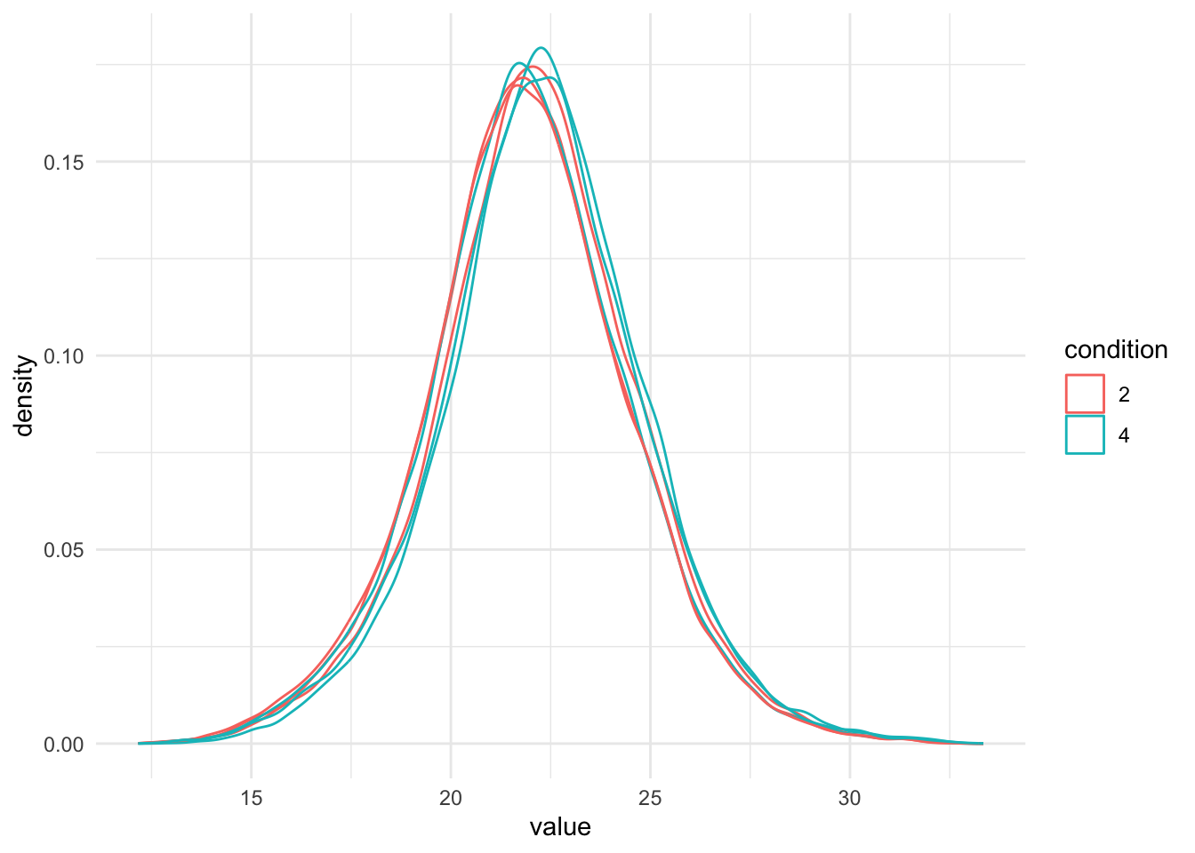
## Normalisation {#sec-norm}
The most common objective of MS-based proteomics experiments is to
understand the biological changes in protein abundance between
experimental conditions. However, changes in measurements between
groups can be caused due to technical factors. For instance, there are
systematic fluctuations from run-to-run that shift the measured
intensity distribution. We can this explore as follows:
1. We extract the sets containing the log transformed data. This is
performed using `QFeatures`' 3-way subsetting.
2. We use `longForm()` to convert the `QFeatures` object into a long
table, including `condition` and `concentration` for filtering and
colouring.
3. We visualise the density of the quantitative values within each
sample. We colour each sample based on its spike-in condition.
```{r}
qf[, , "precursors_log"] |> #1.
  longForm(colvars = colnames(colData(qf))) |>  #2.
  data.frame() |>
  filter(!is.na(value)) |>
  ggplot() + #3.
  aes(x = value,
      colour = condition,
      group = colname) +
  geom_density() +
  theme_minimal()
```
There are many ways to perform the normalisation, e.g. median centering is a popular choice.
If we subtract the sample median at the log scale from each precursor log2 intensity, this basically boils down to calculating log-ratio's between the precursor intensity and its sample median.
Here, we will use the Median of Ratios method of DESeq2, which was originally
developed for RNA-seq data analysis and can also correct for differences in
composition of the proteomes in the different samples.
The method first calculates pseudo-reference sample (row-wise mean of log2
intensities, which corresponds to the log2 transformed geometric mean).
THen calculates log2 ratios of each sample w.r.t. the pseudo-reference.
Finally the column wise median of these log2 ratios is taken to obtain
the sample based normalisation factor on the log2 scale.
This procedure is implemented in the `msqrob2` function `nfLogMedianOfRatios`.
1. We calculate the log transformed normalisation factor from the Median of
Ratios method
2. Subtract these log2-norm factors from the intensities of each corresponding
column of the assay data and store the result in the new assay peptides_norm.
(We adopt the sweep function to the `peptides_log` assay of the spikein
QFeatures object with as statistic the log2 normfactor `STATS = nfLog` the
default function `FUN = "-"`, `MARGIN = 2` to substract the column wise log2
norm factor from each entry of the corresponding assay data).
```{r}
qf <- sweep( #4. Subtract log2 norm factor column-by-column (MARGIN = 2)
  qf,
  MARGIN = 2,
  STATS = nfLogMedianOfRatios(qf,"precursors_log"),
  i = "precursors_log",
  name = "precursors_norm"
)
```
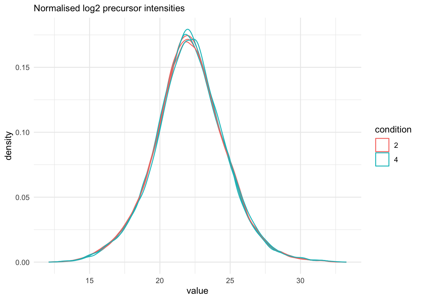
We explore the effect of the global normalisation in the subsequent plot.
Formally, the function applies the following operation on each sample
$i$ across all precursors $p$:
$$
y_{ip}^{\text{norm}} = y_{ip} - \log_2(nf_i)
$$
with $y_ip$ the log2-transformed intensities and $nf_i$ the log2-transformed norm factor. Upon normalisation, we can see
that the distribution of the $y_{ip}^{\text{norm}}$ nicely overlap (using the same code as above)
```{r}
qf[, , "precursors_norm"] |>
  longForm(colvars = colnames(colData(qf))) |>
  data.frame() |>
  filter(!is.na(value)) |>
  ggplot() +
  aes(x = value,
      colour = condition,
      group = colname) +
  geom_density() +
  labs(subtitle = "Normalised log2 precursor intensities") +
  theme_minimal()
```
## Summarisation
Here, we summarise the precursor-level data into protein intensities using maxLFQ.
maxLFQ first calculates all pairwise log ratio's between samples only using their shared precursors.
Particularly, it uses the median of the log ratio's between the shared precursors s, i.e.
$$r_{ij} = median(y_{sj}-y_{si})$$.
Hence, it first eliminates peptide effects.
It then estimates the summaries by solving
$$
\sum_i\sum_j(y^{prot}_j - y^{prot}_i - r_ij)^2
$$
It is implemented in the `maxLFQ` function of the `iq` package.
`aggregateFeatures()` streamlines summarisation. It requires the name
of a `rowData` column to group the precursors into proteins (or
protein groups), here `Protein.Group`. We provide the summarisation
approach through the `fun` argument. Other summarisation methods
are available from the `MsCoreUtils` package, see `?aggregateFeatures`
for a comprehensive list. The function will return a `QFeatures`
object with a new set that we called `proteins`.
```{r, warning=FALSE}
(qf <- aggregateFeatures(
  qf, i = "precursors_norm",
  name = "proteins",
  fcol = "Protein.Group",
  fun = function(X, ...) iq::maxLFQ(X)$estimate
))
```
# Data exploration and QC
Data exploration aims to highlight the main sources of variation in
the data prior to data modelling and can pinpoint to outlying or
off-behaving samples.
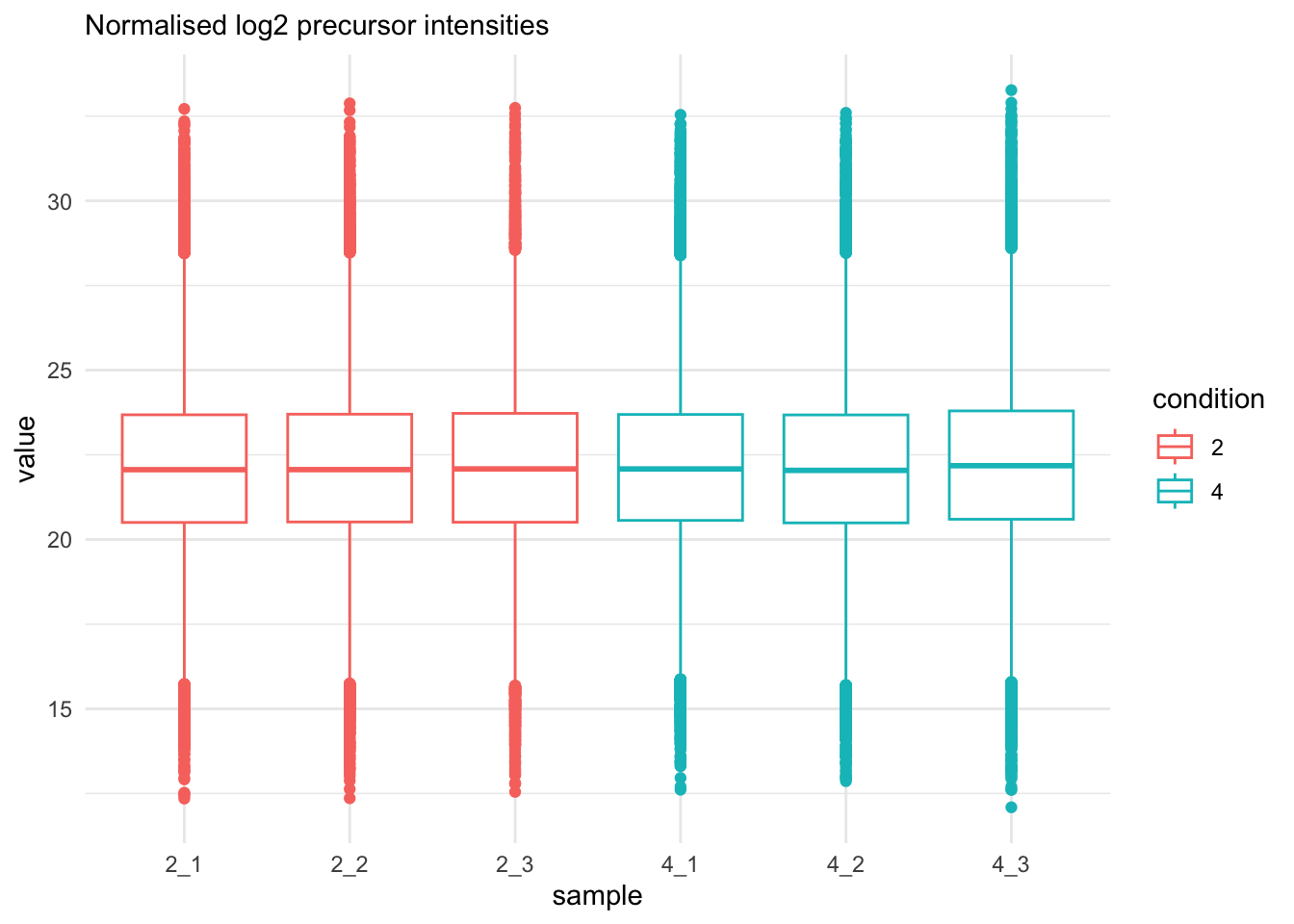
## Marginal distribution at precursor and protein level
```{r}
qf[, , "precursors_norm"] |>
  longForm(colvars = colnames(colData(qf))) |>
  data.frame() |>
  filter(!is.na(value)) |>
  ggplot() +
  aes(x = value,
      colour = condition,
      group = colname) +
  geom_density() +
  theme_minimal() +
   labs(subtitle = "Normalised log2 precursor intensities")
```
```{r}
qf[, , "precursors_norm"] |>
  longForm(colvars = colnames(colData(qf))) |>
  data.frame() |>
  filter(!is.na(value)) |>
  ggplot() +
  aes(x = sampleId,
      y = value,
      colour = condition,
      group = colname) +
  xlab("sample") +
  geom_boxplot() +
  theme_minimal() +
   labs(subtitle = "Normalised log2 precursor intensities")
```
```{r}
qf[, , "proteins"] |>
longForm(colvars = colnames(colData(qf))) |>
data.frame() |>
filter(!is.na(value)) |>
ggplot() +
aes(x = sampleId,
y = value,
colour = condition,
group = colname) +
xlab("sample") +
geom_boxplot() +
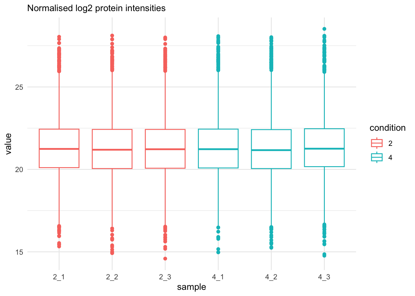
theme_minimal() +
labs(subtitle = "Normalised log2 protein intensities")
```
```{r}
qf[, , "proteins"] |>
longForm(colvars = colnames(colData(qf))) |>
data.frame() |>
filter(!is.na(value)) |>
ggplot() +
aes(x = value,
colour = condition,
group = colname) +
geom_density() +
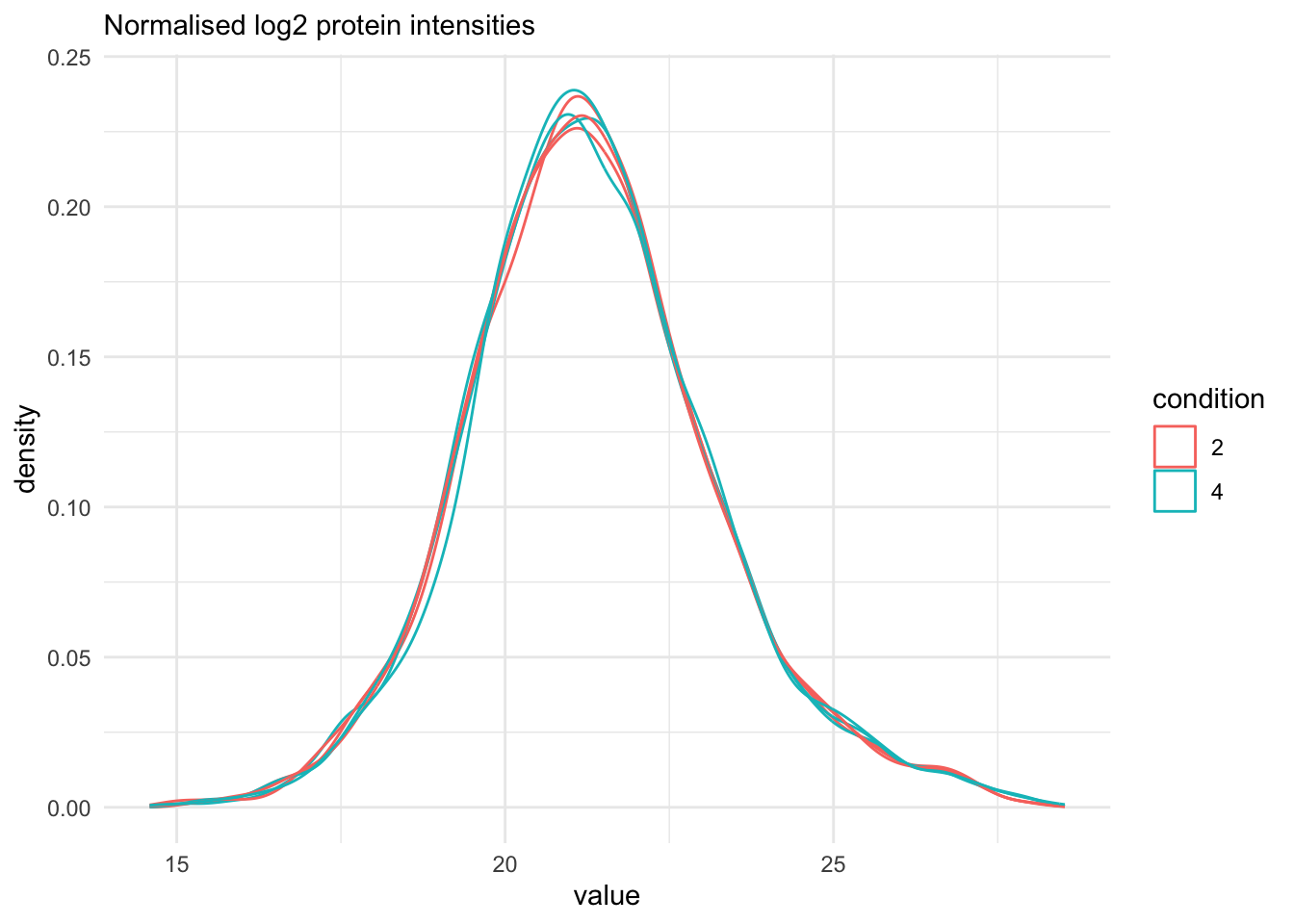
theme_minimal() +
labs(subtitle = "Normalised log2 protein intensities")
```
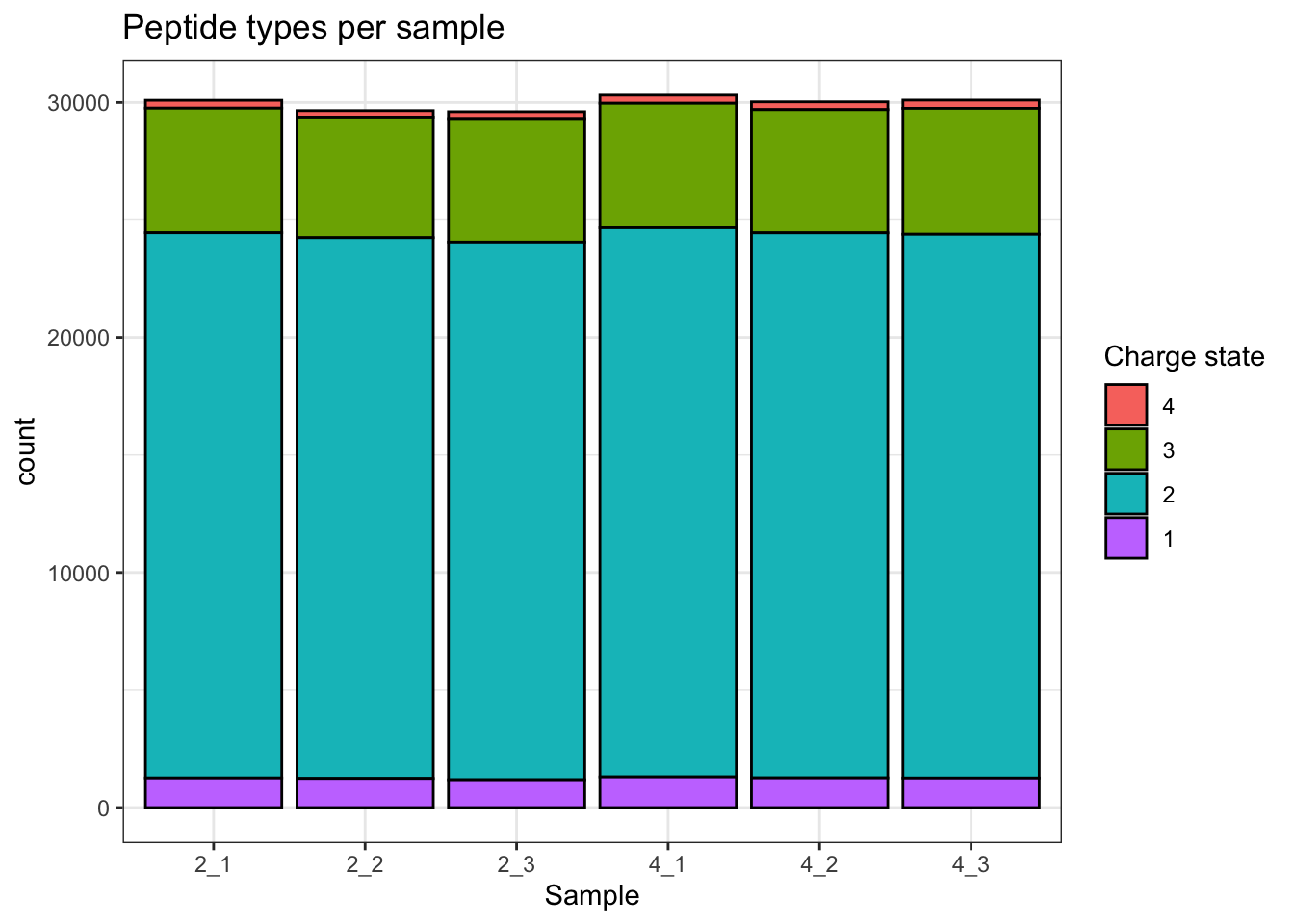
## Charge state
```{r}
qf[, , "precursors_norm"] |>
  longForm(colvars = colnames(colData(qf)), rowvars = "Precursor.Charge") |>
  as.data.frame() |>
  filter(!is.na(value)) |>
  filter(Precursor.Charge<=4) |>
ggplot(aes(x = sampleId)) +
  geom_bar(aes(fill = factor(Precursor.Charge, levels = 4:1)),
           colour = "black") +
  labs(title = "Peptide types per sample",
       x = "Sample",
       fill = "Charge state") +
  theme_bw()
```
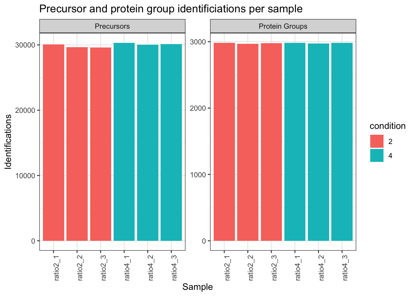
## Identifications per sample
```{r}
qf[,,"precursors_norm"] |>
  longForm(colvars = colnames(colData(qf)),
           rowvars= c("Precursor.Id",
                      "Protein.Group",
                      "Stripped.Sequence",
                      "Precursor.Charge")) |>
  data.frame() |>
  filter(!is.na(value)) |>
  mutate(cond_rep = paste0("ratio", condition, "_", rep)) |>
  group_by(condition, cond_rep) |>
  summarise(Precursors = length(unique(Precursor.Id)),
            `Protein Groups` = length(unique(Protein.Group))) |>
  pivot_longer(-(1:2),
               names_to = "Feature",
               values_to = "IDs") |>
  ggplot(aes(x = cond_rep, y = IDs, fill = condition)) +
  geom_col() +
  #scale_fill_observable() +
  facet_wrap(~Feature,
             scales = "free_y") +
  labs(title = "Precursor and protein group identificiations per sample",
       x = "Sample",
       y = "Identifications") +
  theme_bw() +
  theme(axis.text.x = element_text(angle = 90))
# Data Modeling (Robust Regression){#sec-modelling}
```
## Dimensionality reduction plot
A common approach for data exploration is to
perform dimension reduction, such as Multi Dimensional Scaling (MDS).
We will first extract the set to explore along the sample annotations
(used for plot colouring).
```{r}
se <- getWithColData(qf, "proteins")
```
We then use the `scater` package to compute and plot the PCA. For
technical reasons, it requires `SingleCellExperiment` class object,
but these can easily be generated from a `SummarizedExperiment`
object.
```{r}
se <- runMDS(as(se, "SingleCellExperiment"), exprs_values = 1)
```
We can now explore the data structure while coloring for the factor of
interest, here `condition`.
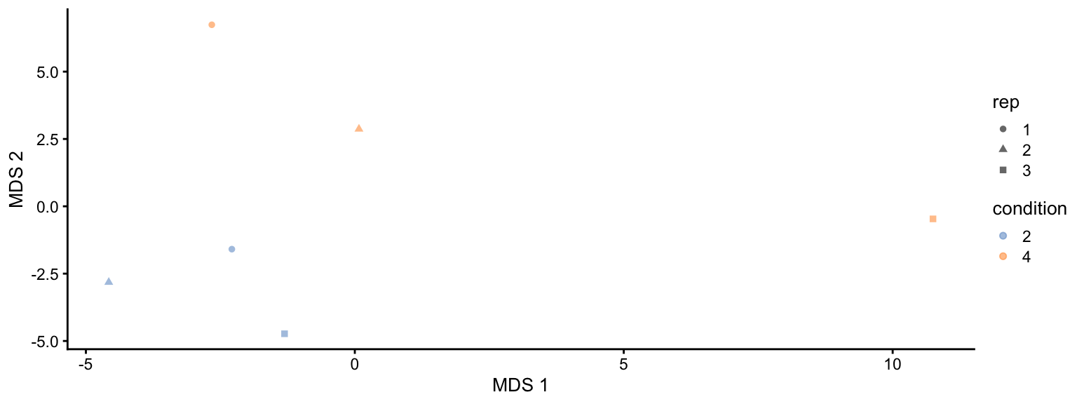
```{r fig.width=8, fig.height=3, fig.cap="MDS visualisation of the spike-in data set. Each point represents a sample and is coloured by the spike-in condiion."}
plotMDS(se, colour_by = "condition", shape_by = "rep")
```
This plot reveals interesting information. First, we see that the
samples are nicely separated according to their spike-in condition.
Interestingly, the conditions are sorted by the concentration.
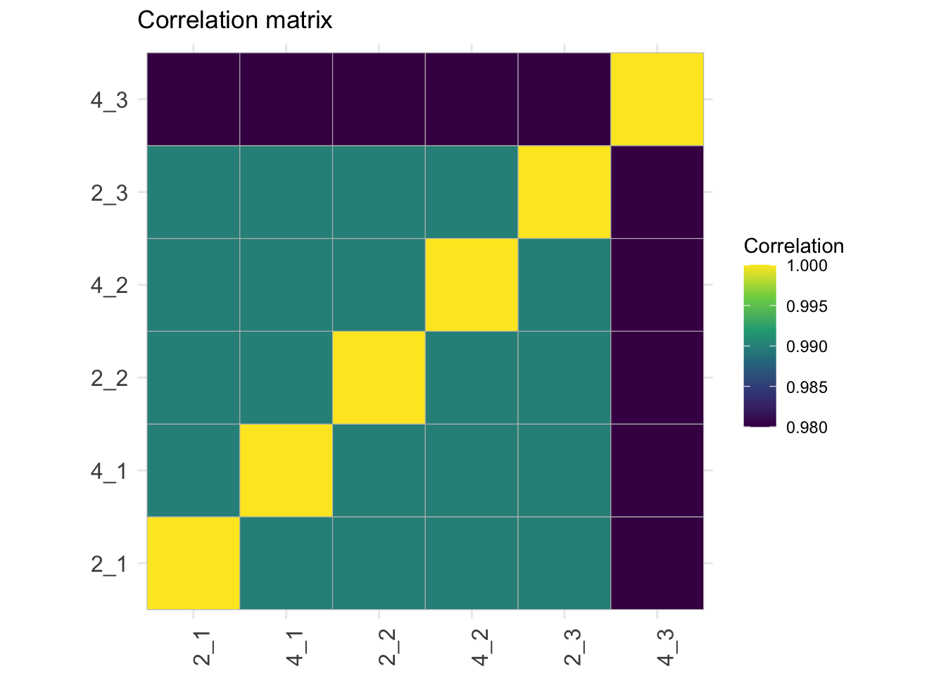
## Correlation matrix
```{r}
corMat <- qf[["proteins"]] |>
  assay() |>
  cor(method = "spearman", use = "pairwise.complete.obs")

colnames(corMat) <- qf$sampleId
rownames(corMat) <- qf$sampleId
corMat |>
  ggcorrplot::ggcorrplot() +
  scale_fill_viridis_c() +
  labs(title = "Correlation matrix",
       fill = "Correlation") +
  theme(axis.text.x = element_text(angle = 90))
```
# Data Modeling (Robust Regression){#sec-modelling}
## Model estimation
1. We first define the model. We only have one sources of variability in the experiment that we can model, i.e. the effect of the spike-in condition.
2. We fit the model to each protein in the `proteins` summarised experiment of the QFeatures object `qf` using the msqrob function.
```{r warning=FALSE}
model <- ~ condition

qf <- msqrob(
  qf,
  i = "proteins",
  formula = model,
  robust = TRUE)
```
We enabled M-estimation (`robust = TRUE`) for improved robustness
against outliers.
The fitting results are available in the `msqrobModels` column of the
`rowData`. More specifically, the modelling output is stored in the
`rowData` as a `statModel` object, one model per row (protein). We
will see in a later section how to perform statistical inference on
the estimated parameters.
```{r}
models <- rowData(qf[["proteins"]])[["msqrobModels"]]
models[1:3]
```
## Inference
We can now convert the research question "do the spike-in
conditions affect the protein intensities?" into a statistical
hypothesis.
In other words, we need to translate this question in a null and alternative hypothesis on a single model parameter or a linear combination of model parameters, which is also referred to with a [contrast](#sec-inference).
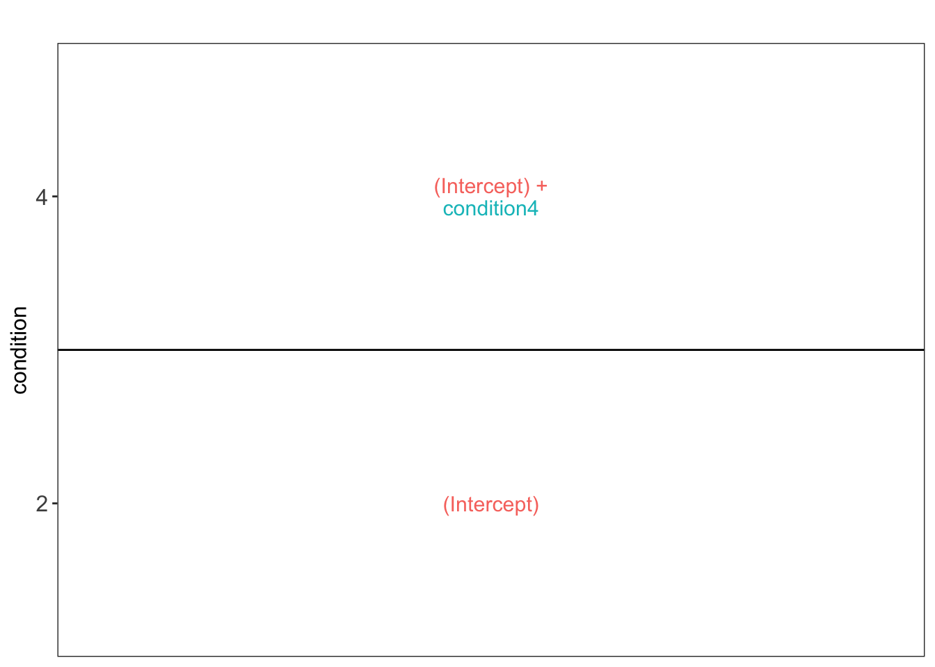
To aid defining contrasts, we will visualise the experimental design using the `ExploreModelMatrix` package.
```{r}
vd <- ExploreModelMatrix::VisualizeDesign(
    sampleData =  colData(qf),
    designFormula = model,
    textSizeFitted = 4
)
vd$plotlist
```
We have a two group comparison and the average log2 fold change between condition 4 and condition 2 can be estimated using parameter:
$$
\log_2 \widehat{\text{FC}}^{4-2} = \hat\mu^4 - \hat\mu^2 = ((Intercept) + condition4) - (Intercept) = condition4
$$
So we can assess the null hypothesis that a protein is not differentially abundant between spike-in condition 4 and spike-in condition 2 as follows
$$
H_0 \log_2 \widehat{\text{FC}}^{4-2} = 0 \text{ or } condition4 = 0
$$
Below we define the contrast and construct the corresponding contrast matrix.
```{r}
contrast <- "condition4 = 0"
(L <- makeContrast(
  contrast,
   parameterNames = colnames(vd$designmatrix)
))
```
We assess the contrast for each protein.
```{r warning=FALSE}
qf <- hypothesisTest(qf, i = "proteins", contrast = L)
```
We extract the results table from the `proteins` summarised experiment in the `qf` object.
```{r}
inference <-
  msqrobCollect(qf[["proteins"]], L)
```
## Report results
We report the results using a results table, volcano plots and heatmaps.
### Results table
We report all results that are significant at the nominal FDR level of 5%.
1. We define the nominal FDR level
2. We filter the results
3. We arrange them according to statistical significance
```{r}
alpha  <- 0.05
inference |>
  filter(adjPval < alpha) |>
  arrange(pval) |>
  knitr::kable()
```
We observe that the results only contain spiked UPS proteins.
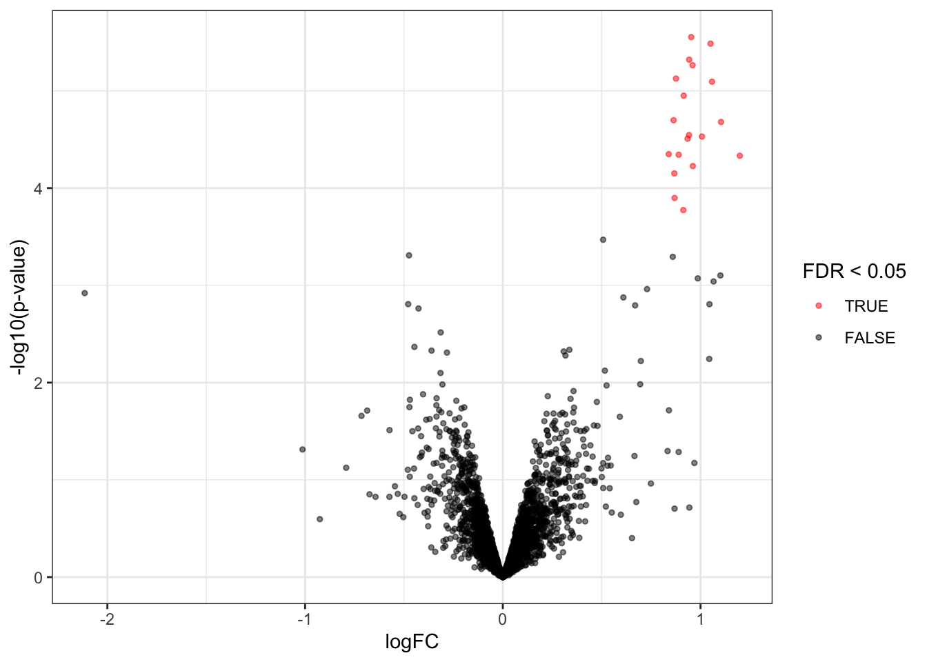
### Volcanoplots
```{r}
volcanoplot4 <- plotVolcano(inference)
volcanoplot4
```
Note, that the log fold changes are nicely around the real log2 fold change: $log2(4/2) = 1$
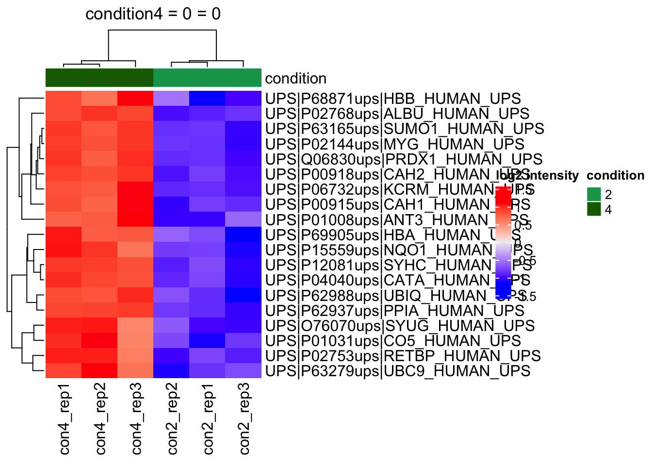
### Heatmaps
We make the heatmap as follows
1. We select the names of the proteins that were declared significant between condition A and condition B and extract their quantitative data.
2. We extract the quantitative data with `assay()` and scale by rows.
3. We will create a heatmap using the ComplexHeatmap package, which enables heatmap annotations. We will annotate the heatmap using our model variables condition and lab.
4. We make the heatmap
```{r}
sig <- inference |>
  filter(adjPval < alpha) |>
  arrange(pval) |>
  pull(feature) #1.

se <- getWithColData(qf, "proteins")
quants <- t(scale(t(assay(se[sig,])))) #2.

colnames(quants) <- paste0("con", se$condition,"_rep",se$rep) #specific to this dataset to get short colnames
annotations <- columnAnnotation(
  condition = se$condition
) #3.

set.seed(1234) ## annotation colours are randomly generated by default
heatmap <- Heatmap(
                       quants,
                       name = "log2 intensity",
                       top_annotation = annotations,
                       column_title = paste0(contrast, " = 0")
                       ) #4.
heatmap
```
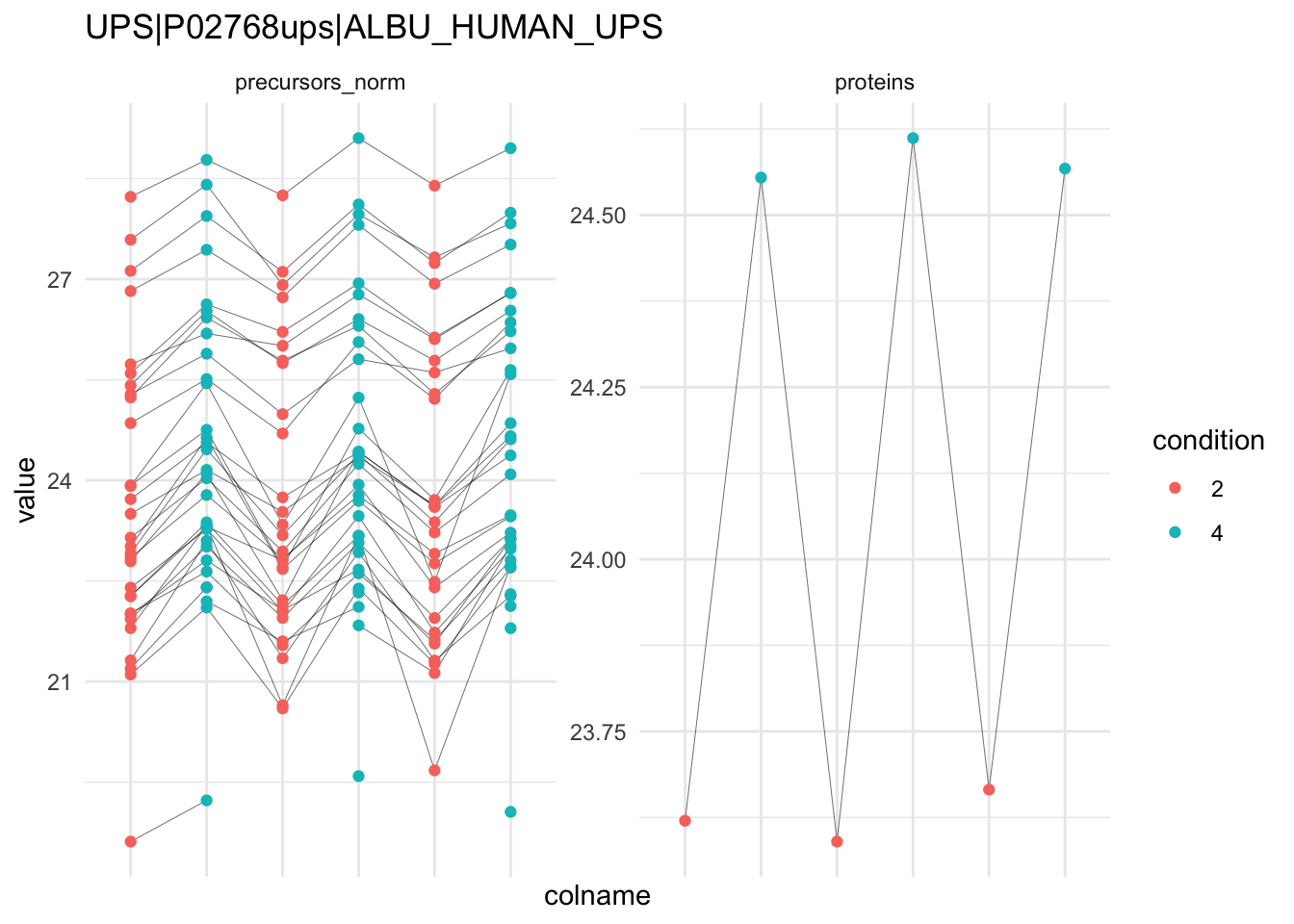
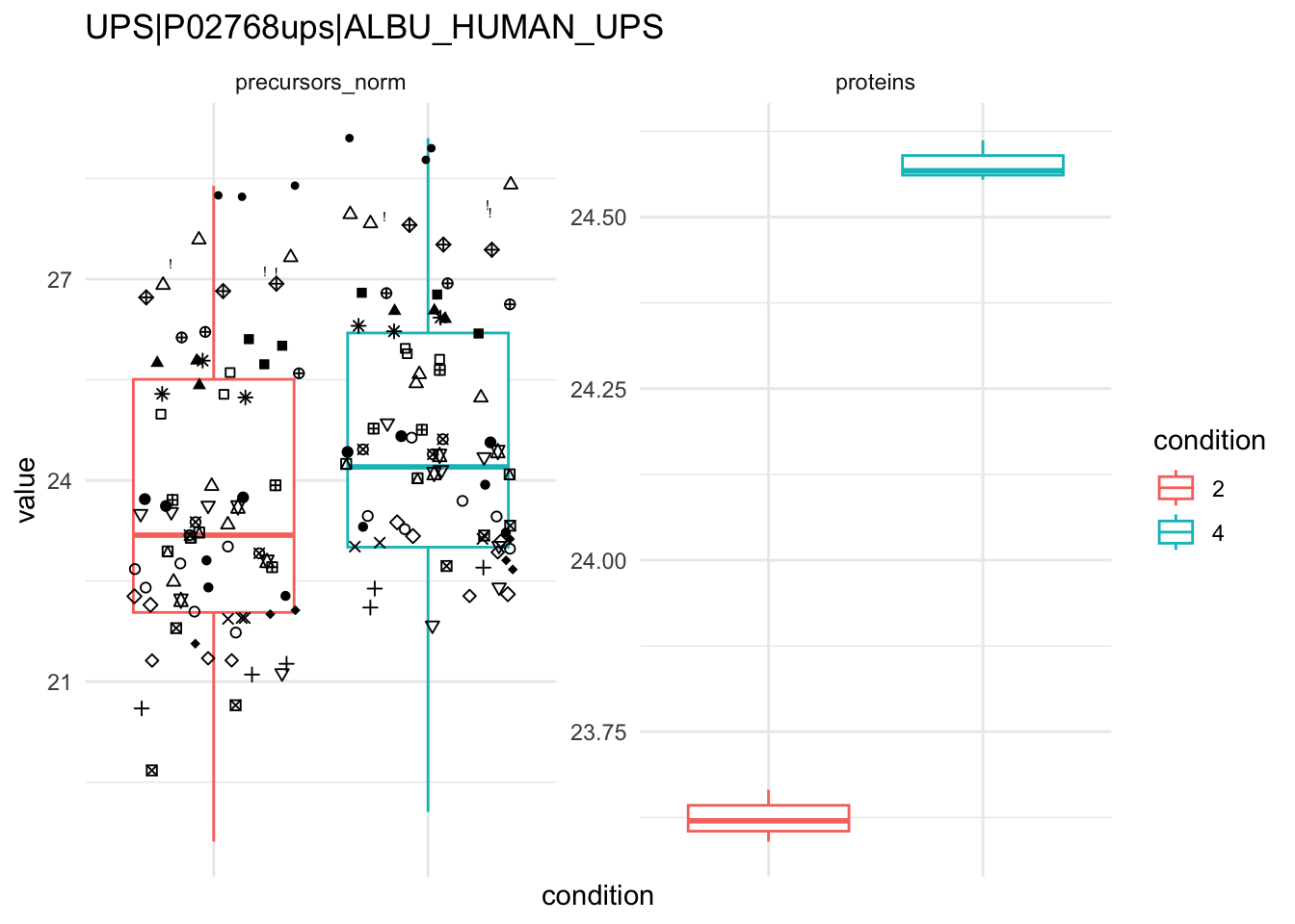
### Detail plots
We can explore the data for a protein to validate the statistical inference results. For example, let’s explore the normalised precursor and the summarised protein intensities for the protein with the most significant log2 fold change.
```{r}
(targetProtein <- inference |>
   slice(which.min(pval)) |>
   pull(feature)
)
```
To obtain the required data, we perform a little data manipulation pipeline:
We use the QFeatures subsetting functionality to retrieve all data related to and focusing on the peptides_log and proteins sets that contains the peptide ion data used for model fitting. We then convert the data with longForm() for plotting. Finally, we plot the log2 normalised intensities for each sample at the protein and at the peptide level. Since multiple peptides are recorded for the protein, we link peptides across samples using a grey line. Samples are colored according to E. coli spike-in condition.
```{r}
qf[targetProtein, , c("precursors_norm", "proteins")] |> #1
  longForm(colvars = colnames(colData(qf))) |> #2
  data.frame() |>
  ggplot() +
  aes(x = colname,
      y = value) +
  geom_line(aes(group = rowname), linewidth = 0.1) +
  geom_point(aes(colour = condition)) +
  facet_wrap(~ assay, scales = "free") +
  ggtitle(targetProtein) +
  theme_minimal() +
  theme(axis.text.x = element_blank())
```
```{r}
qf[targetProtein, , c("precursors_norm", "proteins")] |> #1
  longForm(colvars = colnames(colData(qf))) |> #2
  data.frame() %>%
  {
  ggplot(.) +
  aes(x = condition,
      y = value) +
  geom_boxplot(aes(colour = condition)) +
  facet_wrap(~ assay, scales = "free") +
  geom_jitter(aes(shape = rowname)) +
  scale_shape_manual(values = seq_len(dplyr::n_distinct(.$rowname))) +
  ggtitle(targetProtein) +
  theme_minimal() +
  theme(axis.text.x = element_blank()) +
  guides(shape = "none")
  }
```