---
title: "Introduction to proteomics data analysis - MaxQuant Data Dependent Acquisition spike-in study"
code-tools: true
author:
- name: Lieven Clement, Stijn Vandenbulcke, Oliver M. Crook and Christophe Vanderaa
orcid: 0000-0002-9050-4370
affiliation:
- name: Ghent University
---
# Introduction
Label-Free Quantitative mass spectrometry based workflows for differential
expression (DE) analysis of proteins is often challenging due to
peptide-specific effects and context-sensitive missingness of peptide
intensities.
- `msqrob2` provides peptide-based workflows that can assess for DE directly
from peptide intensities and outperform summarisation methods which first
aggregate MS1 peptide intensities to protein intensities before DE analysis.
However, they are computationally expensive, often hard to understand for the
non-specialised end-user, and they do not provide protein summaries, which are
important for visualisation or downstream processing.
- `msqrob2` therefore also proposes a novel summarisation strategy, which
estimates MSqRob's model parameters in a two-stage procedure circumventing the
drawbacks of peptide-based workflows.
- the summarisation based workflow in `msqrob2` maintains MSqRob's superior
performance, while providing useful protein expression summaries for plotting
and downstream analysis.
Summarising peptide to protein intensities considerably reduces the
computational complexity, the memory footprint and the model complexity.
Moreover, it renders the analysis framework to become modular, providing users
the flexibility to develop workflows tailored towards specific applications.
In this vignette we will demonstrate how to perform `msqrob`'s summarisation
based workflow starting from a Maxquant search on a subset of the cptac
spike-in study.
Examples on our peptide-based workflows and on the analysis of more complex
designs can be found on our companion website
[msqrob2 book](https://statomics.github.io/msqrob2book).
Technical details on our methods can be found in [@goeminne2016],
[@goeminne2020], [@sticker2020] and [@vandenbulcke2025].
# Background
This case-study is a subset of the data of the 6th study of the Clinical
Proteomic Technology Assessment for Cancer (CPTAC).
In this experiment, the authors spiked the Sigma Universal Protein Standard
mixture 1 (UPS1) containing 48 different human proteins in a protein background
of 60 ng/$\mu$L Saccharomyces cerevisiae strain BY4741.
Two different spike-in concentrations were used:
6A (0.25 fmol UPS1 proteins/$\mu$L) and 6B (0.74 fmol UPS1 proteins/$\mu$L) [5].
We limited ourselves to the data of LTQ-Orbitrap W at site 56.
The data were searched with MaxQuant version 1.5.2.8, and
detailed search settings were described in Goeminne et al. (2016) [1].
Three replicates are available for each concentration.
# Load packages
We load the `msqrob2` package, along with additional packages for
data manipulation and visualisation.
```{r load_libraries}
suppressPackageStartupMessages({
library("QFeatures")
library("dplyr")
library("tidyr")
library("ggplot2")
library("msqrob2")
library("stringr")
library("ExploreModelMatrix")
library("kableExtra")
library("ComplexHeatmap")
library("scater")
})
```
# Data
## Peptide table
We first import the data from the peptide.txt file. This is the file containing
your peptide-level intensities searched by MaxQuant search,
this peptide.txt file can be found by default in the
"path_to_raw_files/combined/txt/" folder from the MaxQuant output,
with "path_to_raw_files" the folder where the raw files were saved.
In this vignette, we use a MaxQuant peptide file which is a subset
of the cptac study.
This data is available in
[msqrob2data](https://github.com/statOmics/msqrob2data) GitHub repository.
To import the data we use the `QFeatures` package.
We generate the object peptideFile with the path to the peptide.txt file.
This can be a path to the data on the web or a path to data on your local
computer.
```{r file_location}
peptideFile <- "https://github.com/statOmics/msqrob2data/raw/refs/heads/main/dda/cptacAvsB_lab3/peptides.txt"
```
We will import the data using the `fread` function of the data.table package.
We set the `check.names` argument equal to `TRUE` so that all column names are
retrieved using the `$` operator.
We also use argument integer64 = "double" because `readQFeatures` from the
`QFeatures` package does not process 64-bit integers correctly.
```{r import_data}
peptides <- data.table::fread(peptideFile,
                              check.names = TRUE,
                              integer64 = "double")
head(peptides)
```
Each row in the peptide data table contains information about one peptide
(the table above shows the first 6 rows). The columns contains various
descriptors about the peptide, such as its sequence, its charge, the amino acid
composition, etc. Some of these columns (those starting with `Intensity `)
contain the quantification values for each sample. The table format where the
quantitative values for each sample are contained in a separate column is
depicted as the "wide format", as opposed to the "long format"
(e.g., the [PSM table]).
```{r extract_quantCols}
quantCols <- grep("Intensity[.]", names(peptides), value = TRUE)
```
Unlike for real experiments, we known the ground truth for this dataset: UPS
proteins were spiked in at different concentrations and are thus differentially
abundant (DA, spiked in).
Yeast proteins consist of the background proteome that is the same in all
samples and are thus non-DA.
```{r add_species_info}
peptides <- peptides |>
  mutate(species = grepl(pattern = "UPS",Proteins) |>
           as.factor() |>
           recode("TRUE"="ups","FALSE" = "yeast"))
```
## Sample annotation
Each row in the annotation table contains information about one sample. The
columns contain various descriptors about the sample, such as the name of the
sample or the MS run, the treatment (here the spike-in condition), or any other
biological or technical information that may impact the data quality or the
quantification. Without an annotation table, no analysis can be performed. The
sample annotations are generated by the researcher. In this example, the
annotations are extracted from the sample names, although reporting a detailed
design of experiments in a table is better practice.
1. We first generate a variable quantCols, which contain the names of the
quantification columns.
2. Next we generate variable `sampleId`, to pinpoint the different samples in
the dataset. Since all quantification columns start with the generic string
`Intensity 6` we replace the string with an empty string `""` so we keep the
last 3 characters to refer to the sample.
3. We construct a variable condition, by using the first letter of the
sampleId, which refers to the spikein condition.
4. We construct a variable rep, by using the third letter of the
sampleId.
```{r make_annotation}
(annot <- data.frame(quantCols = quantCols) |> #1.
  mutate(sampleId = gsub("Intensity[.]6","", quantCols), #2.
         condition = substr(sampleId,1,1), #3.
         rep = substr(sampleId, 3, 3)) #4.
)
```
## Convert to QFeatures
The `readQFeatures()` enables a seamless conversion of tabular data into a
`QFeatures` object. We provide the peptide table and the sample annotation table.
The function will use the `quantCols` column in the sample annotation table to
understand which columns in `peptides` contain the quantitative values, and
automatically link the corresponding sample annotation with the quantitative
values. We also tell the function to use the `Sequence` column as peptide
identifier, which will be used as rownames. See `?readQFeatures()` for more
details.
```{r convert_to_QFeatures}
(qf <- readQFeatures(assayData = peptides,
                     colData = annot,
                     name = "peptides",
                     fnames = "Sequence")
)
```
# Data preprocessing
Since we have a `QFeatures` object, we can directly make use of `QFeatures’`
data preprocessing functionality. A major advantage of QFeatures is it provides
the power to build highly modular workflows, where each step is carried out by a
dedicated function with a large choice of available methods and parameters. This
means that users can adapt the workflow to their specific use case and their
specific needs.
## Encoding missing values
The first preprocessing step is to correctly encode the missing values.
It is important that missing values are encoded using `NA`. For instance,
non-observed values should not be encoded with a zero because true zeros
(the proteomic feature is absent from the sample) cannot be distinguished from
technical zeros (the feature was missed by the instrument or could not be
identified). We therefore replace any zero in the quantitative data with an `NA`.
```{r convert0_to_NA}
qf <- zeroIsNA(qf, "peptides") # convert 0 to NA
```
Note that `msqrob2` can handle missing data without having to rely on hard-to-verify imputation assumptions, which is our general recommendation. However, `msqrob2` does not prevent users from using imputation, which can be performed with `impute()` from the QFeatures package.
## $\log_2$ transformation
We perform log2-transformation with `logTransform()` from the `QFeatures`
package.
```{r log2_transformation}
qf <- logTransform(qf, base = 2, i = "peptides", name = "peptides_log")
```
## Peptide-Filtering
Filtering removes low-quality and unreliable peptides that would otherwise introduce noise and artefacts in the data.
### Remove failed protein inference
We remove peptides that could not be mapped to a protein. We also remove peptides that cannot be uniquely mapped to a single proteins because its sequence is shared across multiple proteins. This often occurs for homologs or for proteins that share similar functional domains. Shared peptides are often mapped to protein groups, which are the set of proteins that share the given peptides. Protein groups are encoded by appending the constituting protein identifiers, separated by a `";"`.
```{r failed_protein_inference_filtering}
qf <- filterFeatures(
  qf, ~ Proteins != "" & ## Remove failed protein inference
    !grepl(";", Proteins)) ## Remove protein groups
```
### Remove reverse sequences and contaminants
We now remove the peptides that map to decoy sequences or to
contaminants proteins. In our `peptide.txt`
file decoys and contaminants are indicated with a "+" character in the
column `Reverse` and `Potential.contaminant`, respectively.
Note, that depending on the version of MaxQuant the name of the contaminant variable differs (e.g. `Contaminant` or `Potential contaminant`).
Note, that while reading in the `peptides` table spaces in the column names are replaced by a dot.
```{r filtering_decoys_contaminants}
qf <- filterFeatures(qf, ~ Reverse != "+" & ## Remove decoys
                          Potential.contaminant != "+") ## Remove contaminants
```
### Remove highly missing peptides
The data are characterised by a high proportion of missing values as
reported by `nNA()` from the `QFeatures` package. The function
computes the number and the proportion of missing values across
peptides, samples or for the whole data set and return a list of three
tables called `nNArows`, `nNAcols`, and `nNA`, respectively.
```{r assess_NA_features}
nNaRes <- nNA(qf, "peptides")
range(nNaRes$nNAcols$pNA)
```
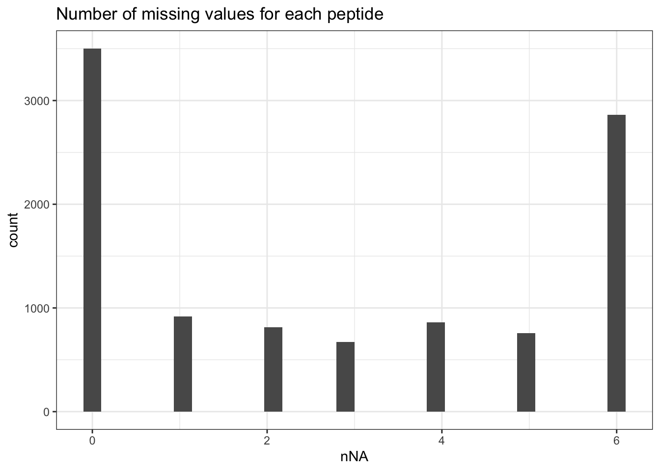
The samples contain between `r round(min(nNaRes$nNAcols$pNA)*100, 1)`%
and `r round(max(nNaRes$nNAcols$pNA)*100, 1)`% missing values. The
missingness within each peptide is more variable, with most peptides
found accross all samples (`nNA` is 0) and other that could not be
quantified in any sample (`nNA` is `r ncol(qf[[1]])`), as depicted
by the histogram below.
```{r plot_NA_features}
data.frame(nNaRes$nNArows) |>
  ggplot() +
  aes(x = nNA) +
  geom_histogram() +
  ggtitle("Number of missing values for each peptide") +
  theme_bw()
```
We keep peptides that were observed at last 3 times out of the $n
= 6$ samples, so that we can estimate the peptide characteristics. We tolerate
the following proportion of NAs:
$\text{pNA} = \frac{(n - 3)}{n} = 0.5$, so we keep peptides that
are observed in at least 50% of the samples, which corresponds to one treatment
condition.
This is an arbitrary value that may need to be adjusted depending on
the experiment and the data set.
```{r filter_features_with_many_NA}
nObs <- 3
n <- ncol(qf[["peptides_log"]])
(qf <- filterNA(qf, i = "peptides_log", pNA = (n - nObs) / n))
```
We keep `r nrow(qf[["peptides_log"]])` peptides upon filtering.
## Normalisation{#sec-norm}
The most common objective of MS-based proteomics experiments is to
understand the biological changes in protein abundance between
experimental conditions. However, changes in measurements between
groups can be caused due to technical factors. For instance, there are
systematic fluctuations from run-to-run that shift the measured
intensity distribution. We can this explore as follows:
1. We extract the sets containing the log transformed data. This is
performed using `QFeatures`' 3-way subsetting.
2. We use `longForm()` to convert the `QFeatures` object into a long
table, including all `colData` for filtering and
colouring.
3. We visualise the density of the quantitative values within each
sample. We colour each sample based on its spike-in condition.
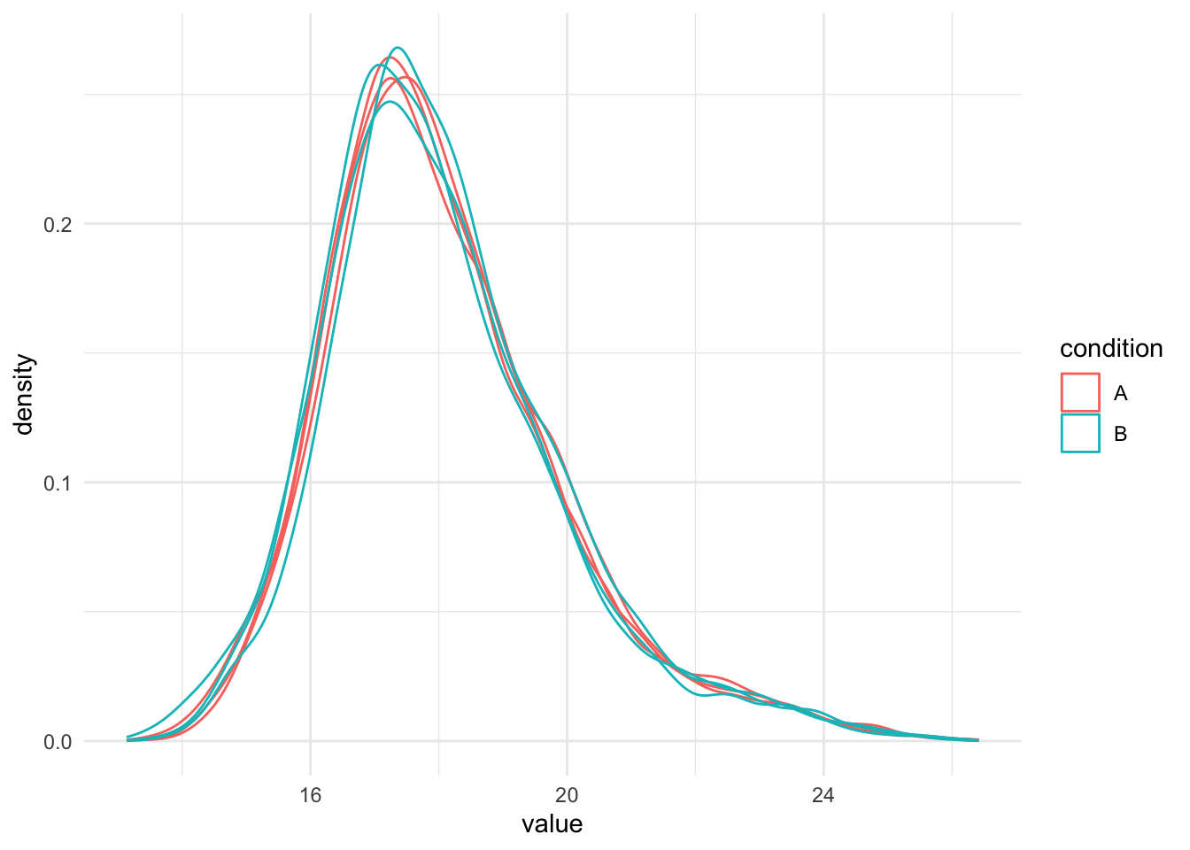
```{r normalisation_needed}
qf[, , "peptides_log"] |> #1.
  longForm(colvars = colnames(colData(qf))) |>  #2.
  data.frame() |>
  filter(!is.na(value)) |>
  ggplot() + #3.
  aes(x = value,
      colour = condition,
      group = colname) +
  geom_density() +
  theme_minimal()
```
Even in this clean synthetic data set (same yeast background with
some spiked UPS proteins), the marginal precursor intensity
distributions across samples are not well aligned. Ignoring this
effect will increase the noise and reduce the statistical power of the
experiment, and may also, in case of unbalanced designs, introduce
confounding effects that will bias the results.
There are many ways to perform the normalisation, e.g.
median centering is a popular choice.
If we subtract the sample median at the log scale from each precursor
log2 intensity, this basically boils down to calculating log-ratio's between
the precursor intensity and its sample median.
Here, we choose to work with offsets, that are chosen in such a way so that
the distributions are centered around the location of a reference sample.
E.g. the median of the sample medians.
Note that users can also use all normalisation functions that are provided in
QFeatures, i.e. by replacing the sweep function by `QFeatures::normalize`.
```{r normalize_peptides}
qf <- sweep( #Subtract log2 norm factor column-by-column (MARGIN = 2)
  qf,
  MARGIN = 2,
  STATS = nfLogMedianOfRatios(qf,"peptides_log"),
  i = "peptides_log",
  name = "peptides_norm"
)
```
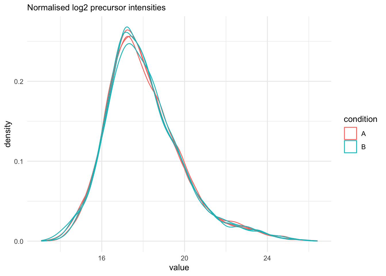
We explore the effect of the global normalisation in the subsequent plot.
Formally, the function applies the following operation on each sample
$i$ across all precursors $p$:
$$
y_{ip}^{\text{norm}} = y_{ip} - \log_2(nf_i)
$$
with $y_{ip}$ the log2-transformed intensities and $\log_2(nf_i)$ the log2-transformed
norm factor. Upon normalisation, we can see that the distribution of the
$y_{ip}^{\text{norm}}$ nicely overlap (using the same code as above)
```{r assess_normalisation}
qf[, , "peptides_norm"] |>
  longForm(colvars = colnames(colData(qf))) |>
  data.frame() |>
  filter(!is.na(value)) |>
  ggplot() +
  aes(x = value,
      colour = condition,
      group = colname) +
  geom_density() +
  labs(subtitle = "Normalised log2 precursor intensities") +
  theme_minimal()
```
## Summarization to protein level
Here, we summarise the peptide-level data into protein intensities using
`aggregateFeatures()`, which streamlines summarisation. It requires the name
of a `rowData` column to group the peptides into proteins (or
protein groups), here `Proteins`. We can provide the summarisation
approach through the `fun` argument.
We use the standard summarisation in aggregateFeatures, which is a
robust summarisation method.
```{r summarize_peptides_to_proteins, warning=FALSE}
qf <- aggregateFeatures(qf,
    i = "peptides_norm",
    fcol = "Proteins",
    na.rm = TRUE,
    name = "proteins"
)
```
Note, that robust summarisation can take a long time for large datasets.
In that case we suggest to use `fun = MsCoreUtils::medianPolish, na.rm = TRUE`.
Note that the optional argument na.rm = TRUE is needed when using `medianPolish`
because the data contains missing values as we did not adopt imputation and
`medianPolish` by default cannot handle missing values.
# Data exploration and QC
Data exploration aims to highlight the main sources of variation in
the data prior to data modelling and can pinpoint to outlying or
off-behaving samples.
## Marginal distribution at precursor and protein level
```{r qc_normalisation_peptides}
qf[, , "peptides_norm"] |>
  longForm(colvars = colnames(colData(qf))) |>
  data.frame() |>
  filter(!is.na(value)) |>
  ggplot() +
  aes(x = value,
      colour = condition,
      group = colname) +
  geom_density() +
  theme_minimal() +
   labs(subtitle = "Normalised log2 precursor intensities")
```
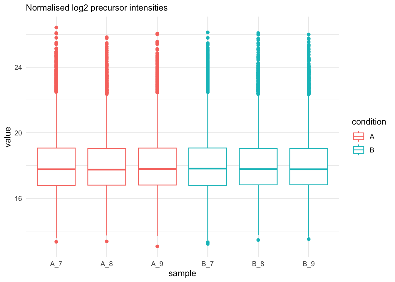
```{r qc_normalisation_peptides_boxplot}
qf[, , "peptides_norm"] |>
  longForm(colvars = colnames(colData(qf))) |>
  data.frame() |>
  filter(!is.na(value)) |>
  ggplot() +
  aes(x = sampleId,
      y = value,
      colour = condition,
      group = colname) +
  xlab("sample") +
  geom_boxplot() +
  theme_minimal() +
   labs(subtitle = "Normalised log2 precursor intensities")
```
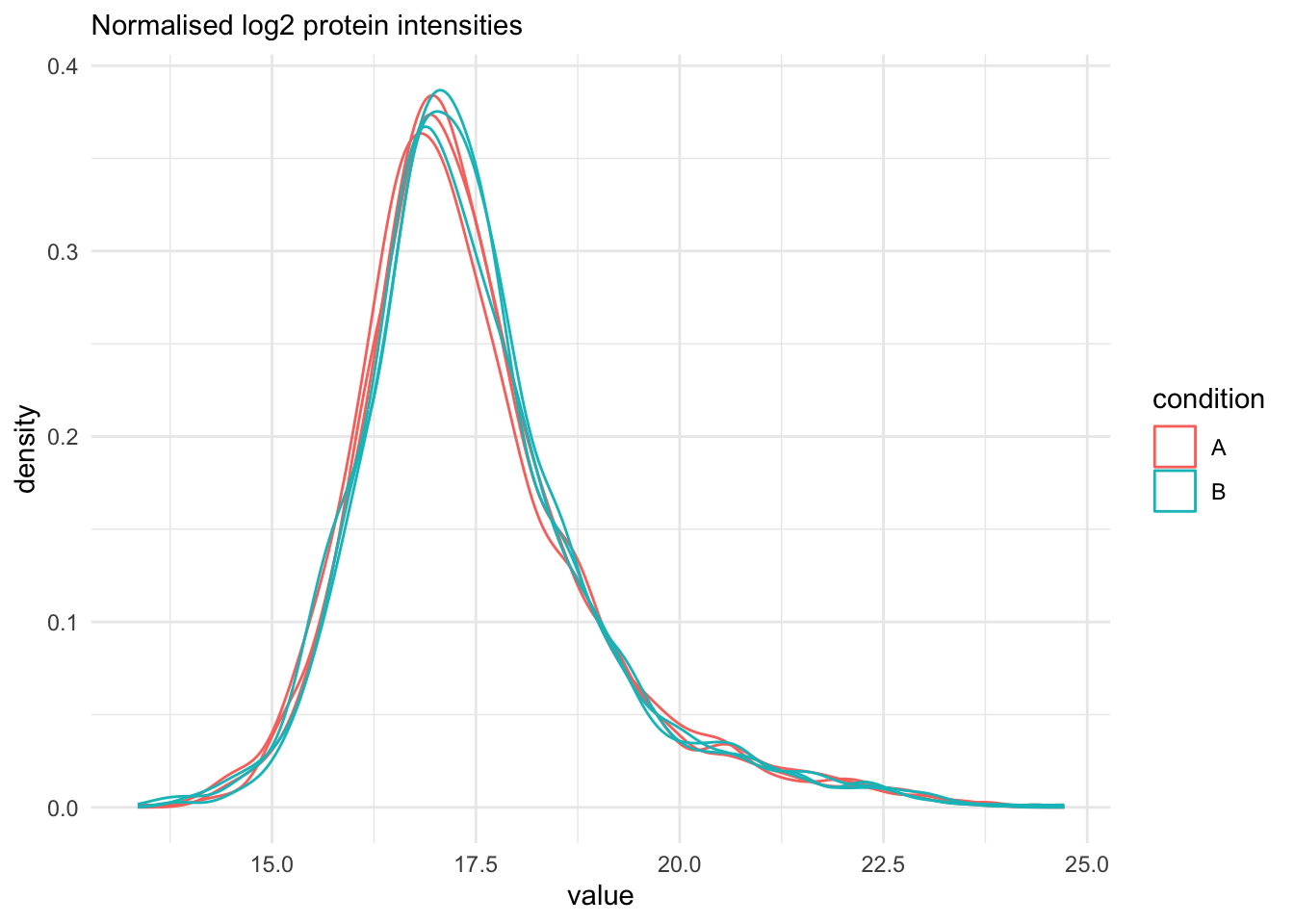
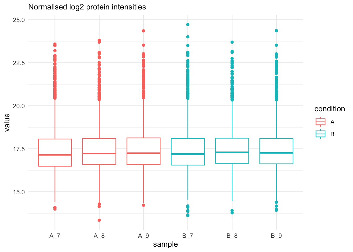
We do the same for the protein-level values.
```{r qc_normalisation_proteins}
qf[, , "proteins"] |>
  longForm(colvars = colnames(colData(qf))) |>
  data.frame() |>
  filter(!is.na(value)) |>
  ggplot() +
  aes(x = value,
      colour = condition,
      group = colname) +
  geom_density() +
  theme_minimal() +
   labs(subtitle = "Normalised log2 protein intensities")
```
```{r qc_normalisation_proteins_boxplot}
qf[, , "proteins"] |>
  longForm(colvars = colnames(colData(qf))) |>
  data.frame() |>
  filter(!is.na(value)) |>
  ggplot() +
  aes(x = sampleId,
      y = value,
      colour = condition,
      group = colname) +
  xlab("sample") +
  geom_boxplot() +
  theme_minimal() +
   labs(subtitle = "Normalised log2 protein intensities")
```
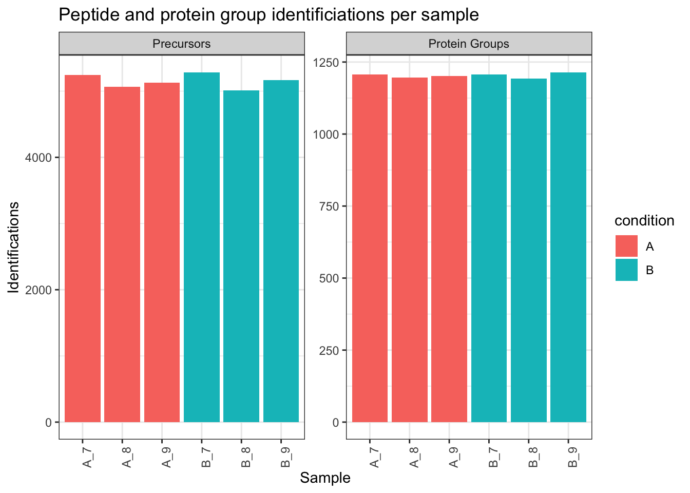
## Identifications per sample
```{r qc_identifications}
qf[,,"peptides_norm"] |>
  longForm(colvars = colnames(colData(qf)),
           rowvars= c("Sequence",
                      "Proteins")) |>
  data.frame() |>
  filter(!is.na(value)) |>
  group_by(condition, sampleId) |>
  summarise(Precursors = length(unique(Sequence)),
            `Protein Groups` = length(unique(Proteins))) |>
  pivot_longer(-(1:2),
               names_to = "Feature",
               values_to = "IDs") |>
  ggplot(aes(x = sampleId, y = IDs, fill = condition)) +
  geom_col() +
  #scale_fill_observable() +
  facet_wrap(~Feature,
             scales = "free_y") +
  labs(title = "Peptide and protein group identificiations per sample",
       x = "Sample",
       y = "Identifications") +
  theme_bw() +
  theme(axis.text.x = element_text(angle = 90))
```
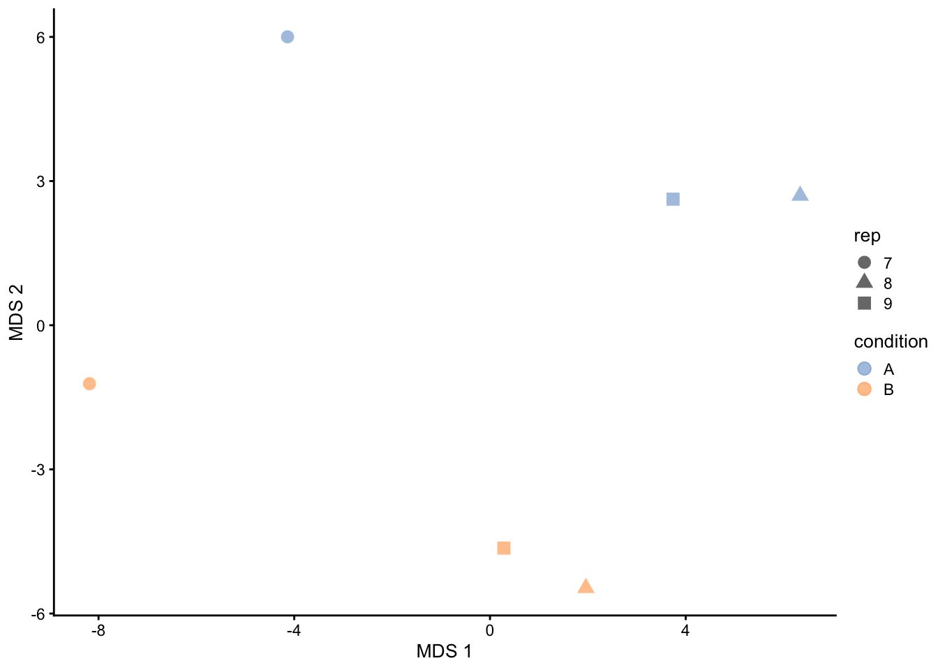
## Dimensionality reduction plot
A common approach for data exploration is to
perform dimension reduction, such as Multi Dimensional Scaling (MDS).
We will first extract the set to explore along the sample annotations
(used for plot colouring).
```{r qc_mds_proteins}
getWithColData(qf, "proteins") |>
  as("SingleCellExperiment") |>
  runMDS(exprs_values = 1) |>
  plotMDS(colour_by = "condition", shape_by = "rep", point_size = 3)
```
This plot reveals interesting information. First, we see that the
samples are nicely separated according to their spike-in condition.
The also seem to line up according to `rep`.
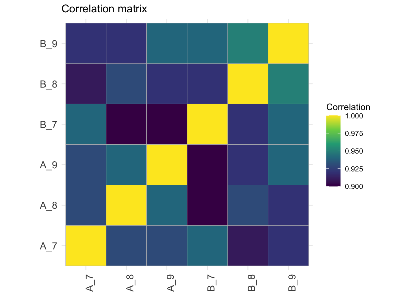
## Correlation matrix
```{r qc_correlation_proteins}
corMat <- qf[["proteins"]] |>
  assay() |>
  cor(method = "spearman", use = "pairwise.complete.obs")

colnames(corMat) <- qf$sampleId
rownames(corMat) <- qf$sampleId
corMat |>
  ggcorrplot::ggcorrplot() +
  scale_fill_viridis_c() +
  labs(title = "Correlation matrix",
       fill = "Correlation") +
  theme(axis.text.x = element_text(angle = 90))
```
# Data Modeling (Robust Regression){#sec-modelling}
## Sources of variation
For this experiment, we can only model a single source of variation: spike-in
concentration. All remaining sources of variability, e.g. pipetting errors,
MS run to run variability, etc will be lumped in the residual variability
(error term).
Spike-in condition effects: we model the source of variation induced by the
experimental treatment of interest as a fixed effect, which we consider
non-random, i.e. the treatment effect is assumed to be the same in repeated
experiments, but it is unknown and has to be estimated.
When modelling a typical label-free experiment at the protein level, the model
boils down to the following linear model:
$$ y_i = \mathbf{x}_i^T\boldsymbol{\beta} +\epsilon_i$$
with the $\log_2$-normalised and summarised protein intensities in sample;
$\mathbf{x}_i$ a vector with the covariate pattern for the sample encoding the
intercept, spike-in condition, or other experimental factors;
$\boldsymbol{\beta}$ the vector of parameters that model the association between
the covariates and the outcome; and $\epsilon_i$ the residuals reflecting
variation that is not captured by the fixed effects.
Note that allows for a flexible parameterisation of the treatment
beyond a single covariate, i.e. including a 1 for the intercept, continuous and
categorical variables as well as their interactions. We assume the residuals to
be independent and identically distributed (i.i.d) according to a normal
distribution with zero mean and constant variance,
i.e. $\epsilon_i \sim N(0, \sigma^2_\epsilon)$, that can differ from protein to
protein.
In R, this model is encoded using the following simple formula:
```{r define_model}
model <- ~ condition
```
## Model Estimation
We estimate the model with `msqrob()`. The function takes the QFeatures object,
extracts the quantitative values from the `"proteins"` set generated during
summarisation, and fits a simple linear model with `condition` as covariate,
which are automatically retrieved from `colData(qf)`.
Note, that `msqrob()` can also take a `SummarizedExperiment` of
precursor, peptide or protein intensities as its input.
```{r fit_models, warning=FALSE}
  qf <- msqrob(
    qf,
    i = "proteins",
    formula = model,
    robust = TRUE)
```
We enable M-estimation (`robust = TRUE`) for improved robustness against outliers.
The fitting results are available in the `msqrobModels` column of the rowData. More specifically, the modelling output is stored in the `rowData` as a `statModel` object, one model per row (protein). We will see in a later section how to perform statistical inference on the estimated parameters.
```{r print_models}
models <- rowData(qf[["proteins"]])[["msqrobModels"]]
models[1:3]
```
## Statistical inference
We can now convert the research question “do the spike-in conditions affect the protein intensities?” into a statistical hypothesis.
In other words, we need to translate this question in a null and alternative hypothesis on a single model parameter or on a linear combination of model parameters, which is also referred to with a contrast.
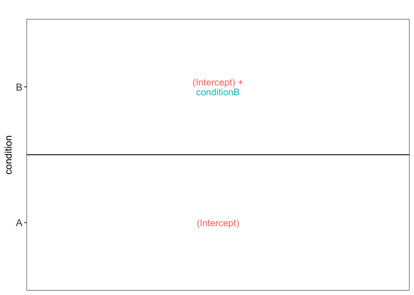
To aid defining contrasts, we will visualise the experimental design using the `ExploreModelMatrix` package.
```{r explore_model_matrix}
vd <- ExploreModelMatrix::VisualizeDesign(
    sampleData =  colData(qf),
    designFormula = model,
    textSizeFitted = 4
)
vd$plotlist
```
This plot shows that the average protein $\log_2$ intensity for conditionA is modelled by `(Intercept)` and that for the `conditionB` group by `(Intercept) + conditionB` .
Hence, to assess differential abundance of proteins between the two spike-in conditions, we will have to assess the following null hypothesis: $\log_2 FC_{B-A} = (Intercept + conditionB) - Intercept = conditionB = 0$.
Based on this null hypothesis we now generate a contrast matrix.
```{r make_contrasts}
(L <- makeContrast(
  "conditionB = 0",
  parameterNames = colnames(vd$designmatrix)
))
```
We can now test our null hypothesis using `hypothesisTest()` which
takes the `QFeatures` object with the fitted model and the contrast we
just built. `msqrob2` automatically applies the hypothesis
testing to all features in the assay.
```{r hypthesis_tests}
qf <- hypothesisTest(qf, i = "proteins", contrast = L)
```
The results tables for the contrast are stored in the row data of the
`proteins` assay in `qf` under the colomnames of the contrast matrix `L`.
Users can directly access the results tables via de colData. However, `msqrob2`
also provides the `msqrobCollect` function. This function will automatically
retrieve the results tables for all contrasts in contrast matrix `L` and combine
them by default in one table. This table contains two additional columns:
`contrast` with the name of the contrast and `feature` with the name of the
modelled `feature`, here protein.
```{r collect_results}
inferences <-
  msqrobCollect(qf[["proteins"]], L)
head(inferences)
```
### Results table for significant proteins
We will return a table of proteins for which the contrast is significant at the 5% FDR level.
1. We set the significance level
3. We filter the significant results for the contrast from the table
4. We print the table
```{r significant_table, results='asis'}
alpha <- 0.05 #1.
sigList <- inferences |>
    filter(adjPval < alpha) #3.
kable(sigList) |>
      kable_styling(full_width = FALSE) |>
      scroll_box(height = "250px") #4.
```
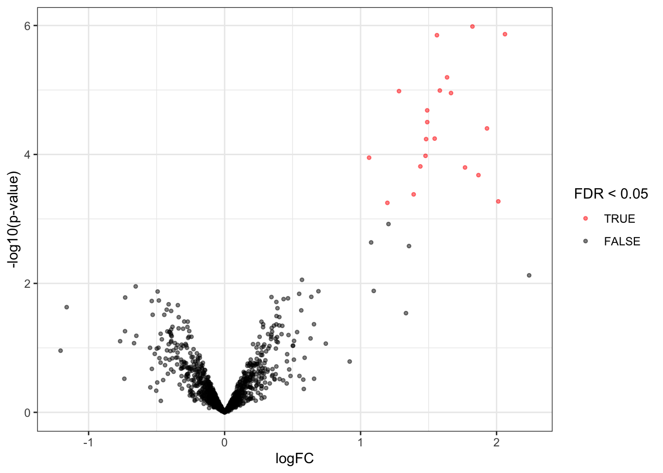
### Volcanoplots
A volcano plot is a common visualisation that provides an overview of
the hypothesis testing results, plotting the $-\log_{10}$ p-value^[Note,
that upon this transformation a value of 1 represents a p-value of 0.1, 2
a p-value of 0.01, 3 a p-value of 0.001, etc.] as a function of
the estimated log fold change. Volcano plots can be used to highlight
the most interesting proteins that have large fold changes and/or are
highly significant. We can use the table above directly to build a
volcano plot using `ggplot2` functionality. We also highlight which
proteins are UPS standards, known to be differentially abundant by
experimental design.
Experienced users can make the plot themselves. However, in msqrob2 we also
provide the plotVolcano function that generates volcanoplots based on `msqrob2`
inference tables generated with the `hypothesisTest` function.
```{r volcanoplot}
inferences |>
  plotVolcano()
```
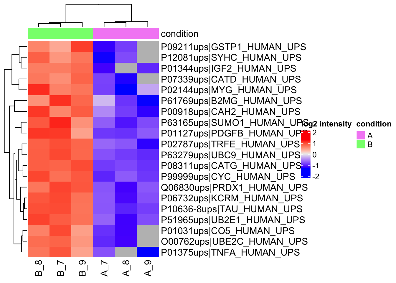
### Heatmaps
We construct heatmaps for the significant proteins for each contrast.
1. We get the names of the significant features.
2. We extract the quant data for the significant features and scale it.
3. We extract annotation
4. We make the heatmap using the quants data. We do not cluster columns (samples) to keep them together according to the design.
```{r heatmap}
sig <- sigList |> pull(feature) #1.


quants <- assay(qf,"proteins")[sig,] |>
                     t() |>
                     scale() |>
                     t() #2.

colnames(quants) <- qf$sampleId #3.
annotations <- columnAnnotation(condition = qf$condition) #3.

set.seed(1234) ## annotation colours are randomly generated by default
Heatmap(
  quants,
  name = "log2 intensity",
  top_annotation = annotations
  )  #4.
```
Note, that `r nrow(sigList)` DA proteins are returned and that they are all UPS proteins!
A typical workflow for the analysis of a proteomics experiment will end here.
# References
Note, that more examples can be found in our [msqrob2 book](https://statomics.github.io/msqrob2book).
```{r sessionInfo}
sessionInfo()
```