Statistical Methods for Quantitative MS-based Proteomics: Blocking - Wrap-up

This is part of the online course Proteomics Data Analysis (PDA)

1 Import Data and Preprocessing

1.1 Data

Click to see code

library(tidyverse)
library(limma)
library(QFeatures)
library(msqrob2)
library(plotly)
library(ggplot2)
library(data.table)
library(gridExtra)

peptidesTable <- fread("https://raw.githubusercontent.com/statOmics/PDA21/data/quantification/mouseTcell/peptidesRCB.txt")
int64 <- which(sapply(peptidesTable,class) == "integer64")
for (j in int64) peptidesTable[[j]] <- as.numeric(peptidesTable[[j]]) 

peptidesTable2 <- fread("https://raw.githubusercontent.com/statOmics/PDA21/data/quantification/mouseTcell/peptidesCRD.txt")
int64 <- which(sapply(peptidesTable2,class) == "integer64")
for (j in int64) peptidesTable2[[j]] <- as.numeric(peptidesTable2[[j]]) 

peptidesTable3 <- fread("https://raw.githubusercontent.com/statOmics/PDA21/data/quantification/mouseTcell/peptides.txt")
int64 <- which(sapply(peptidesTable3,class) == "integer64")
for (j in int64) peptidesTable3[[j]] <- as.numeric(peptidesTable3[[j]]) 

quantCols <- grep("Intensity ", names(peptidesTable))
pe <- readQFeatures(
  assayData = peptidesTable,
  fnames = 1,
  quantCols =  quantCols,
  name = "peptideRaw")
rm(peptidesTable)
gc()

##            used  (Mb) gc trigger  (Mb) limit (Mb) max used  (Mb)
## Ncells  8497634 453.9   12240530 653.8         NA 12240530 653.8
## Vcells 44722037 341.3   73581861 561.4      16384 73581855 561.4

gc()

##            used  (Mb) gc trigger  (Mb) limit (Mb) max used  (Mb)
## Ncells  8497612 453.9   12240530 653.8         NA 12240530 653.8
## Vcells 44715558 341.2   73581861 561.4      16384 73581855 561.4

quantCols2 <- grep("Intensity ", names(peptidesTable2))
pe2 <- readQFeatures(
  assayData = peptidesTable2,
  fnames = 1,
  quantCols =  quantCols2,
  name = "peptideRaw")
rm(peptidesTable2)
gc()

##            used  (Mb) gc trigger  (Mb) limit (Mb) max used  (Mb)
## Ncells  8409494 449.2   12240530 653.8         NA 12240530 653.8
## Vcells 38110740 290.8   73581861 561.4      16384 73581855 561.4

gc()

##            used  (Mb) gc trigger  (Mb) limit (Mb) max used  (Mb)
## Ncells  8409493 449.2   12240530 653.8         NA 12240530 653.8
## Vcells 38106457 290.8   73581861 561.4      16384 73581855 561.4

quantCols3 <- grep("Intensity ", names(peptidesTable3))
pe3 <- readQFeatures(
  assayData = peptidesTable3,
  fnames = 1,
  quantCols =  quantCols3,
  name = "peptideRaw")
rm(peptidesTable3)
gc()

##            used  (Mb) gc trigger  (Mb) limit (Mb) max used  (Mb)
## Ncells  8409080 449.1   12240530 653.8         NA 12240530 653.8
## Vcells 29422356 224.5   73581861 561.4      16384 73581855 561.4

gc()

##            used  (Mb) gc trigger  (Mb) limit (Mb) max used  (Mb)
## Ncells  8409005 449.1   12240530 653.8         NA 12240530 653.8
## Vcells 29417798 224.5   73581861 561.4      16384 73581855 561.4

### Design
colData(pe)$celltype <- substr(
  colnames(pe[["peptideRaw"]]),
  11,
  14) |>
  unlist() |>  
  as.factor()

colData(pe)$mouse <- pe[[1]] |>
  colnames() |>
  strsplit(split="[ ]")  |>
  sapply(function(x) x[3]) |>
  as.factor()

colData(pe2)$celltype <- substr(
  colnames(pe2[["peptideRaw"]]),
  11,
  14) |>
  unlist() |>  
  as.factor()

colData(pe2)$mouse <- pe2[[1]] |>
  colnames() |>
  strsplit(split="[ ]")  |>
  sapply(function(x) x[3]) |>
  as.factor()

colData(pe3)$celltype <- substr(
  colnames(pe3[["peptideRaw"]]),
  11,
  14) |>
  unlist() |>  
  as.factor()

colData(pe3)$mouse <- pe3[[1]] |>
  colnames() |>
  strsplit(split="[ ]")  |>
  sapply(function(x) x[3]) |>
  as.factor()

1.2 Preprocessing

1.2.0.1 Log-transform

Click to see code to log-transfrom the data

• Peptides with zero intensities are missing peptides and should be represent with a NA value rather than 0.

pe <- zeroIsNA(pe, "peptideRaw") # convert 0 to NA

pe2 <- zeroIsNA(pe2, "peptideRaw") # convert 0 to NA

pe3 <- zeroIsNA(pe3, "peptideRaw") # convert 0 to NA

• Logtransform data with base 2

pe <- logTransform(pe, base = 2, i = "peptideRaw", name = "peptideLog")

pe2 <- logTransform(pe2, base = 2, i = "peptideRaw", name = "peptideLog")

pe3 <- logTransform(pe3, base = 2, i = "peptideRaw", name = "peptideLog")

1.2.1 Filtering

Click to see details on filtering

1. Remove peptides that map to multiple proteins

We remove PSMs that could not be mapped to a protein or that map to multiple proteins (the protein identifier contains multiple identifiers separated by a ;).

pe <- filterFeatures(
    pe, ~ Proteins != "" & ## Remove failed protein inference
        !grepl(";", Proteins)) ## Remove protein groups

## 'Proteins' found in 2 out of 2 assay(s).

pe2 <- filterFeatures(
    pe2, ~ Proteins != "" & ## Remove failed protein inference
        !grepl(";", Proteins)) ## Remove protein groups

## 'Proteins' found in 2 out of 2 assay(s).

pe3 <- filterFeatures(
    pe3, ~ Proteins != "" & ## Remove failed protein inference
        !grepl(";", Proteins)) ## Remove protein groups

## 'Proteins' found in 2 out of 2 assay(s).

2. Remove reverse sequences (decoys) and contaminants

We now remove the contaminants, peptides that map to decoy sequences, and proteins which were only identified by peptides with modifications.

pe <- filterFeatures(pe,~Reverse != "+")

## 'Reverse' found in 2 out of 2 assay(s).

pe <- filterFeatures(pe,~ Potential.contaminant != "+")

## 'Potential.contaminant' found in 2 out of 2 assay(s).

pe2 <- filterFeatures(pe2,~Reverse != "+")

## 'Reverse' found in 2 out of 2 assay(s).

pe2 <- filterFeatures(pe2,~ Potential.contaminant != "+")

## 'Potential.contaminant' found in 2 out of 2 assay(s).

pe3 <- filterFeatures(pe3,~Reverse != "+")

## 'Reverse' found in 2 out of 2 assay(s).

pe3 <- filterFeatures(pe3,~ Potential.contaminant != "+")

## 'Potential.contaminant' found in 2 out of 2 assay(s).

3. Drop peptides that were identified in less than three sample

We keep peptides that were observed at least three times.

nObs <- 3
n <- ncol(pe[["peptideLog"]])
pNA <- (n-nObs)/n
pe <- filterNA(pe, pNA = pNA, i = "peptideLog")
nrow(pe[["peptideLog"]])

## [1] 38782

n <- ncol(pe2[["peptideLog"]])
pNA <- (n-nObs)/n
pe2 <- filterNA(pe2, pNA = pNA, i = "peptideLog")
nrow(pe2[["peptideLog"]])

## [1] 37898

n <- ncol(pe3[["peptideLog"]])
pNA <- (n-nObs)/n
pe3 <- filterNA(pe3, pNA = pNA, i = "peptideLog")
nrow(pe3[["peptideLog"]])

## [1] 43984

1.2.2 Normalization

Click to see code to normalize the data

pe <- normalize(pe, 
                i = "peptideLog", 
                name = "peptideNorm", 
                method = "center.median")

pe2 <- normalize(pe2, 
                i = "peptideLog", 
                name = "peptideNorm", 
                method = "center.median")


pe3 <- normalize(pe3, 
                i = "peptideLog", 
                name = "peptideNorm", 
                method = "center.median")

1.2.3 Summarization

Click to see code to summarize the data

pe <- aggregateFeatures(pe,
 i = "peptideNorm",
 fcol = "Proteins",
 na.rm = TRUE,
 name = "protein")

## Your quantitative and row data contain missing values. Please read the
## relevant section(s) in the aggregateFeatures manual page regarding the
## effects of missing values on data aggregation.

## Aggregated: 1/1

pe2 <- aggregateFeatures(pe2,
 i = "peptideNorm",
 fcol = "Proteins",
 na.rm = TRUE,
 name = "protein")

## Your quantitative and row data contain missing values. Please read the
## relevant section(s) in the aggregateFeatures manual page regarding the
## effects of missing values on data aggregation.
## Aggregated: 1/1

pe3 <- aggregateFeatures(pe3,
 i = "peptideNorm",
 fcol = "Proteins",
 na.rm = TRUE,
 name = "protein")

## Your quantitative and row data contain missing values. Please read the
## relevant section(s) in the aggregateFeatures manual page regarding the
## effects of missing values on data aggregation.
## Aggregated: 1/1

1.2.4 Filtering proteins with too many missing values

We want to have at least two observed protein intensities for each group so we set the minimum number of observed values at 4. We still have to check for the observed proteins if that is the case.

For block design more clever filtering can be used. E.g. we could imply that we have both cell types in at least two animals…

nObs <- 4
n <- ncol(pe[["protein"]])
pNA <- (n-nObs)/n
pe<- filterNA(pe, pNA = pNA, i = "protein")

n <- ncol(pe2[["protein"]])
pNA <- (n-nObs)/n
pe2 <- filterNA(pe2, pNA = pNA, i = "protein")

n <- ncol(pe3[["protein"]])
pNA <- (n-nObs)/n
pe3 <- filterNA(pe3, pNA = pNA, i = "protein")

1.3 Data Exploration: what is impact of blocking?

Click to see code

levels(colData(pe3)$mouse) <- paste0("m",1:7)
mdsObj3 <- plotMDS(assay(pe3[["protein"]]), plot = FALSE)
mdsOrig <- colData(pe3) %>%
  as.data.frame %>%
  mutate(mds1 = mdsObj3$x,
         mds2 = mdsObj3$y,
         lab = paste(mouse,celltype,sep="_")) %>%
  ggplot(aes(x = mds1, y = mds2, label = lab, color = celltype, group = mouse)) +
  geom_text(show.legend = FALSE) +
  geom_point(shape = 21) +
  geom_line(color = "black", linetype = "dashed") +
  xlab(
    paste0(
      mdsObj3$axislabel,
      " ",
      1, 
      " (",
      paste0(
        round(mdsObj3$var.explained[1] *100,0),
        "%"
        ),
      ")"
      )
    ) +
  ylab(
    paste0(
      mdsObj3$axislabel,
      " ",
      2, 
      " (",
      paste0(
        round(mdsObj3$var.explained[2] *100,0),
        "%"
        ),
      ")"
      )
    ) +
  ggtitle("Original (RCB)")

levels(colData(pe)$mouse) <- paste0("m",1:4)
mdsObj <- plotMDS(assay(pe[["protein"]]), plot = FALSE)
mdsRCB <- colData(pe) %>%
  as.data.frame %>%
  mutate(mds1 = mdsObj$x,
         mds2 = mdsObj$y,
         lab = paste(mouse,celltype,sep="_")) %>%
  ggplot(aes(x = mds1, y = mds2, label = lab, color = celltype, group = mouse)) +
  geom_text(show.legend = FALSE) +
  geom_point(shape = 21) +
  geom_line(color = "black", linetype = "dashed") +
  xlab(
    paste0(
      mdsObj$axislabel,
      " ",
      1, 
      " (",
      paste0(
        round(mdsObj$var.explained[1] *100,0),
        "%"
        ),
      ")"
      )
    ) +
  ylab(
    paste0(
      mdsObj$axislabel,
      " ",
      2, 
      " (",
      paste0(
        round(mdsObj$var.explained[2] *100,0),
        "%"
        ),
      ")"
      )
    ) +
  ggtitle("Randomized Complete Block (RCB)")


levels(colData(pe2)$mouse) <- paste0("m",1:8)
mdsObj2 <- plotMDS(assay(pe2[["protein"]]), plot = FALSE)
mdsCRD <- colData(pe2) %>%
  as.data.frame %>%
  mutate(mds1 = mdsObj2$x,
         mds2 = mdsObj2$y,
         lab = paste(mouse,celltype,sep="_")) %>%
  ggplot(aes(x = mds1, y = mds2, label = lab, color = celltype, group = mouse)) +
  geom_text(show.legend = FALSE) +
  geom_point(shape = 21) +
  xlab(
    paste0(
      mdsObj$axislabel,
      " ",
      1, 
      " (",
      paste0(
        round(mdsObj2$var.explained[1] *100,0),
        "%"
        ),
      ")"
      )
    ) +
  ylab(
    paste0(
      mdsObj$axislabel,
      " ",
      2, 
      " (",
      paste0(
        round(mdsObj2$var.explained[2] *100,0),
        "%"
        ),
      ")"
      )
    ) +
  ggtitle("Completely Randomized Design (CRD)")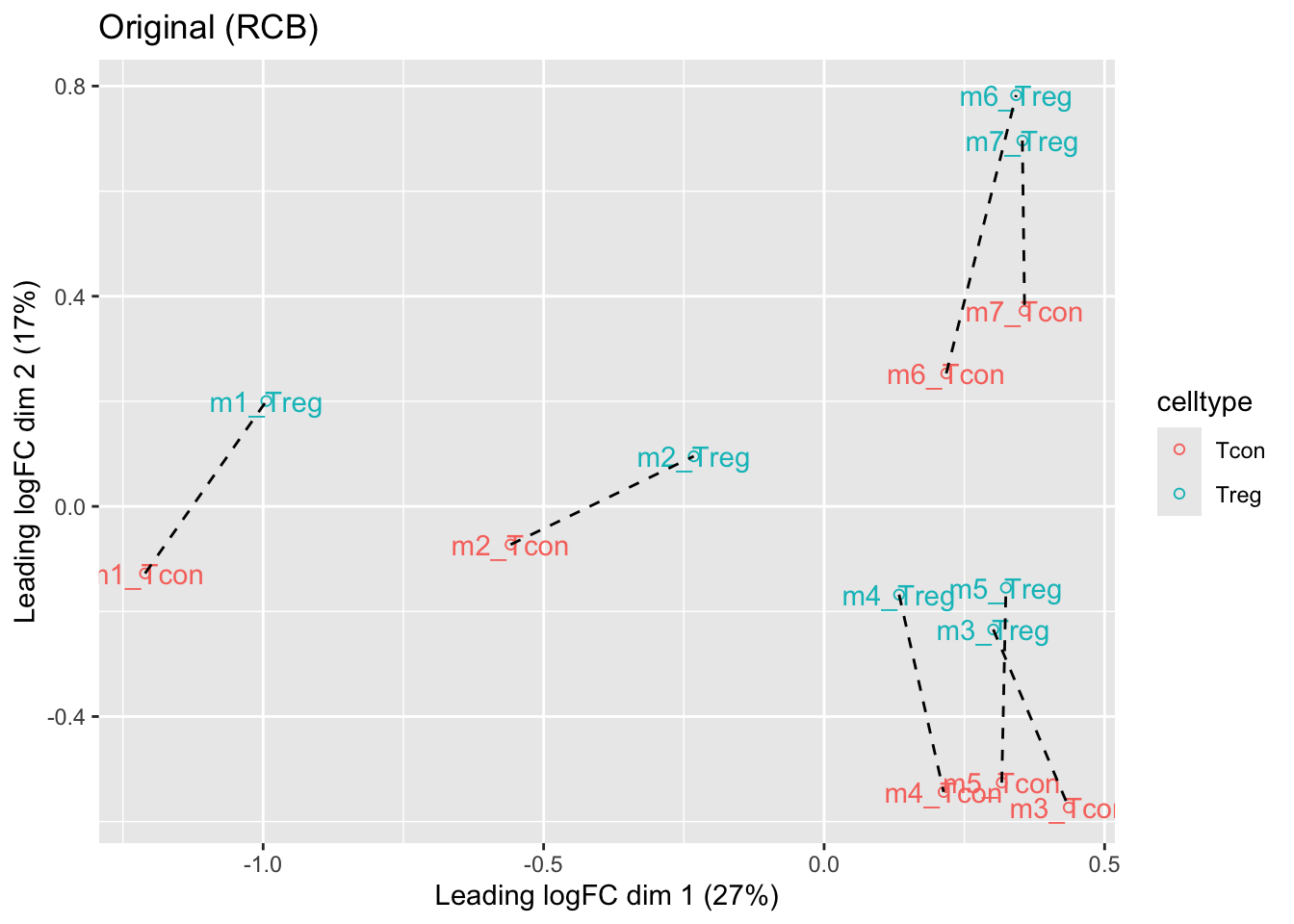

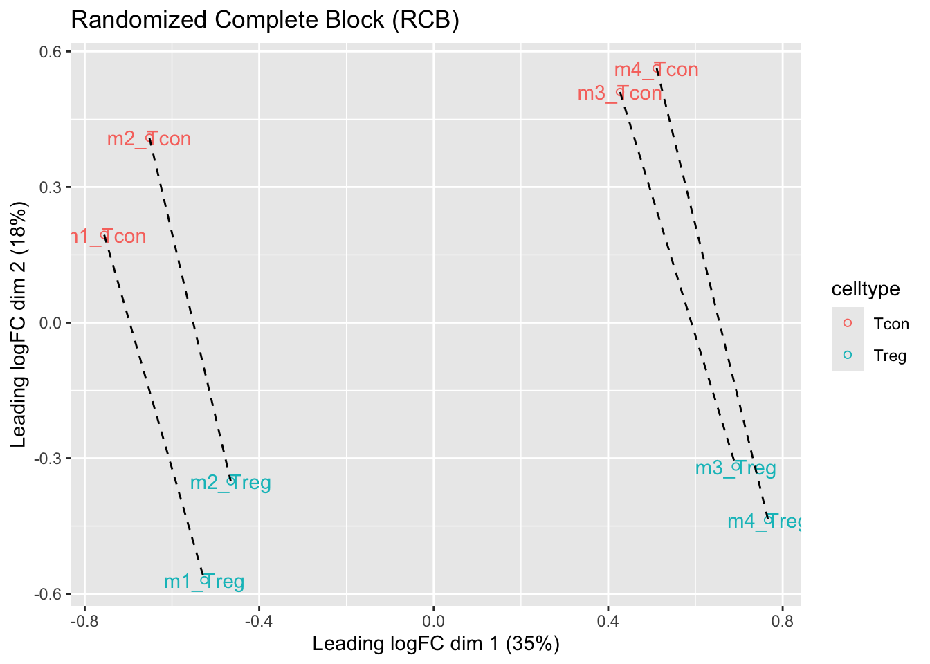
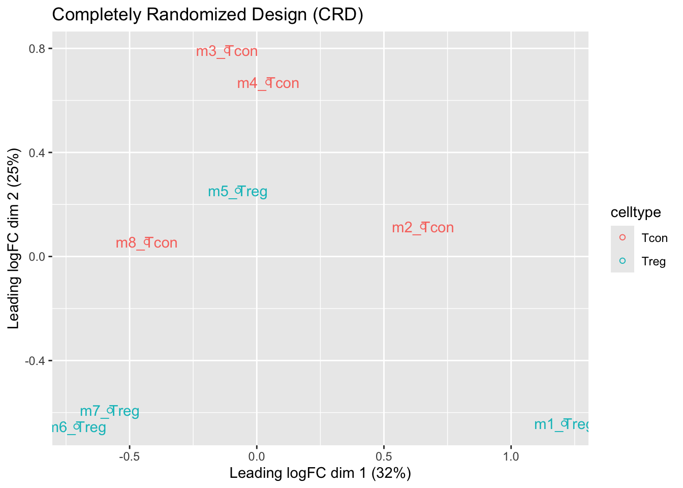
mdsOrig

mdsRCB

mdsCRD

• We observe that the leading fold change is according to mouse
• In the second dimension we see a separation according to cell-type
• With the Randomized Complete Block design (RCB) we can remove the mouse effect from the analysis!

1.4 Modeling and inference

1.4.1 RCB analysis

pe <- msqrob(
  object = pe,
  i = "protein",
  formula = ~ celltype + mouse)

1.4.2 RCB wrong analysis

pe <- msqrob(
  object = pe,
  i = "protein",
  formula = ~ celltype, modelColumnName = "wrongModel")

1.5 CRD analysis

pe2 <- msqrob(
  object = pe2,
  i = "protein",
  formula = ~ celltype)

1.5.1 Inference

library(ExploreModelMatrix)
VisualizeDesign(colData(pe),~ celltype + mouse)$plotlist

## [[1]]

VisualizeDesign(colData(pe2),~ celltype)$plotlist

## [[1]]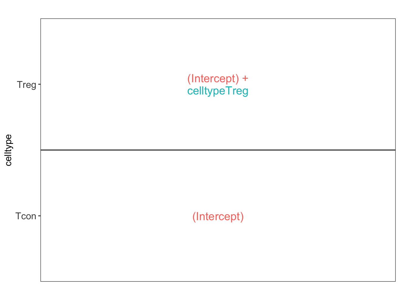

L <- makeContrast("celltypeTreg = 0", parameterNames = c("celltypeTreg"))
pe <- hypothesisTest(object = pe, i = "protein", contrast = L)
pe <- hypothesisTest(object = pe, i = "protein", contrast = L, modelColumn = "wrongModel", resultsColumnNamePrefix="wrong")
pe2 <- hypothesisTest(object = pe2, i = "protein", contrast = L)

2 Advantage of Blocking: comparison between designs

2.1 Volcano plots

Click to see code

volcanoRCB <- ggplot(
    rowData(pe[["protein"]])$celltypeTreg,
    aes(x = logFC, y = -log10(pval), color = adjPval < 0.05)
) +
    geom_point(cex = 2.5) +
    scale_color_manual(values = alpha(c("black", "red"), 0.5)) +
    theme_minimal() +
    ggtitle(paste0("RCB: \n", 
                sum(rowData(pe[["protein"]])$celltypeTreg$adjPval<0.05,na.rm=TRUE),
            " significant"))

volcanoRCBwrong <- ggplot(
    rowData(pe[["protein"]])$wrongcelltypeTreg,
    aes(x = logFC, y = -log10(pval), color = adjPval < 0.05)
) +
    geom_point(cex = 2.5) +
    scale_color_manual(values = alpha(c("black", "red"), 0.5)) +
    theme_minimal() +
    ggtitle(paste0("RCB wrong: \n", 
                sum(rowData(pe[["protein"]])$wrongcelltypeTreg$adjPval<0.05,na.rm=TRUE),
            " significant"))

volcanoCRD <- ggplot(
    rowData(pe2[["protein"]])$celltypeTreg,
    aes(x = logFC, y = -log10(pval), color = adjPval < 0.05)
) +
    geom_point(cex = 2.5) +
    scale_color_manual(values = alpha(c("black", "red"), 0.5)) +
    theme_minimal() +
    ggtitle(paste0("CRD: \n", 
                sum(rowData(pe2[["protein"]])$celltypeTreg$adjPval<0.05,na.rm=TRUE),
            " significant"))

grid.arrange(volcanoRCB,volcanoCRD, volcanoRCBwrong,ncol=2)

## Warning: Removed 453 rows containing missing values or values outside the scale range
## (`geom_point()`).

## Warning: Removed 133 rows containing missing values or values outside the scale range
## (`geom_point()`).

## Warning: Removed 55 rows containing missing values or values outside the scale range
## (`geom_point()`).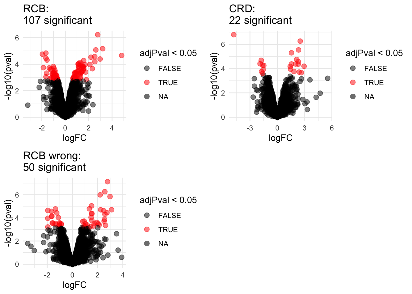

2.2 Anova table: Q7TPR4, Alpha-actinin-1

Disclaimer: the Anova analysis is only for didactical purposes. In practice we assess the hypotheses using msqrob2.

• We illustrate the power gain of blocking using an Anova analysis on 1 protein.

• Note, that msqrob2 will perform a similar analysis, but, it uses robust regression and it uses an empirical Bayes estimator for the variance.

prot <- "Q7TPR4"
dataHlp <- colData(pe) %>% 
  as.data.frame %>%
  mutate(intensity=assay(pe[["protein"]])[prot,],
         intensityCRD=assay(pe2[["protein"]])[prot,])

  anova(lm(intensity~ celltype + mouse, dataHlp)) 

## Analysis of Variance Table
## 
## Response: intensity
##           Df Sum Sq Mean Sq F value    Pr(>F)    
## celltype   1 5.4816  5.4816 483.074 0.0002062 ***
## mouse      3 0.4275  0.1425  12.557 0.0332459 *  
## Residuals  3 0.0340  0.0113                      
## ---
## Signif. codes:  0 '***' 0.001 '**' 0.01 '*' 0.05 '.' 0.1 ' ' 1

  anova(lm(intensity~ celltype,dataHlp))

## Analysis of Variance Table
## 
## Response: intensity
##           Df Sum Sq Mean Sq F value    Pr(>F)    
## celltype   1 5.4816  5.4816  71.264 0.0001508 ***
## Residuals  6 0.4615  0.0769                      
## ---
## Signif. codes:  0 '***' 0.001 '**' 0.01 '*' 0.05 '.' 0.1 ' ' 1

  anova(lm(intensityCRD~ celltype,dataHlp))

## Analysis of Variance Table
## 
## Response: intensityCRD
##           Df Sum Sq Mean Sq F value    Pr(>F)    
## celltype   1 5.3495  5.3495  61.763 0.0002245 ***
## Residuals  6 0.5197  0.0866                      
## ---
## Signif. codes:  0 '***' 0.001 '**' 0.01 '*' 0.05 '.' 0.1 ' ' 1

2.3 Comparison Empirical Bayes standard deviation in msqrob2

Click to see code

accessions <- rownames(pe[["protein"]])[rownames(pe[["protein"]])%in%rownames(pe2[["protein"]])]
dat <- data.frame(
sigmaRBC = sapply(rowData(pe[["protein"]])$msqrobModels[accessions], getSigmaPosterior),
sigmaRBCwrong = sapply(rowData(pe[["protein"]])$wrongModel[accessions], getSigmaPosterior),
sigmaCRD <- sapply(rowData(pe2[["protein"]])$msqrobModels[accessions], getSigmaPosterior)
)

 plotRBCvsWrong <- ggplot(data = dat, aes(sigmaRBC, sigmaRBCwrong)) +
    geom_point(alpha = 0.1, shape = 20) +
    scale_x_log10() +
    scale_y_log10() +
    geom_abline(intercept=0,slope=1)
plotCRDvsWrong <- ggplot(data = dat, aes(sigmaCRD, sigmaRBCwrong)) +
    geom_point(alpha = 0.1, shape = 20) +
    scale_x_log10() +
    scale_y_log10() +
    geom_abline(intercept=0,slope=1)
plotRBCvsCRD <- ggplot(data = dat, aes(sigmaRBC, sigmaCRD)) +
    geom_point(alpha = 0.1, shape = 20) +
    scale_x_log10() +
    scale_y_log10() +
    geom_abline(intercept=0,slope=1)

grid.arrange(
  plotRBCvsWrong,
  plotCRDvsWrong,
  plotRBCvsCRD,
  nrow=2)

## Warning: Removed 316 rows containing missing values or values outside the scale range
## (`geom_point()`).

## Warning: Removed 124 rows containing missing values or values outside the scale range
## (`geom_point()`).

## Warning: Removed 351 rows containing missing values or values outside the scale range
## (`geom_point()`).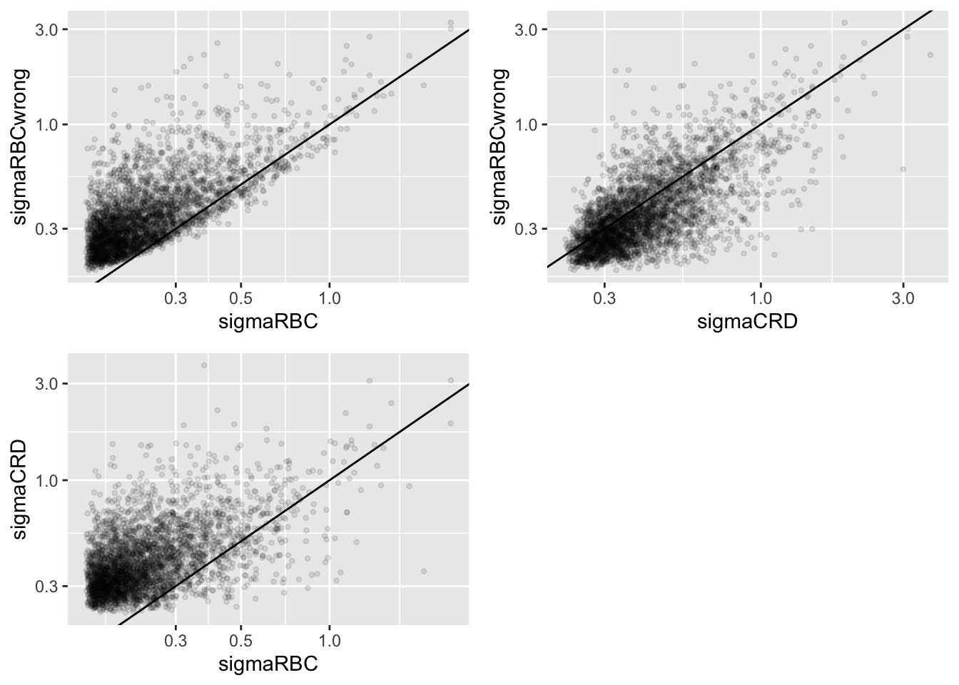

• We clearly observe that the standard deviation of the protein expression in the RCB is smaller for the majority of the proteins than that obtained with the CRD

• The standard deviation of the protein expression RCB where we perform a wrong analysis without considering the blocking factor according to mouse is much larger for the marjority of the proteins than that obtained with the correct analysis.

• Indeed, when we ignore the blocking factor in the RCB design we do not remove the variability according to mouse from the analysis and the mouse effect is absorbed in the error term. The standard deviation than becomes very comparable to that observed in the completely randomised design where we could not remove the mouse effect from the analysis.

• Why are some of the standard deviations for the RCB with the correct analysis larger than than of the RCB with the incorrect analysis that ignored the mouse blocking factor?

• Can you think of a reason why it would not be useful to block on a particular factor?