Introduction to proteomics data analysis: robust summarization

This is part of the online course Proteomics Data Analysis (PDA)

1 Background

This case-study is a subset of the data of the 6th study of the Clinical Proteomic Technology Assessment for Cancer (CPTAC). In this experiment, the authors spiked the Sigma Universal Protein Standard mixture 1 (UPS1) containing 48 different human proteins in a protein background of 60 ng/\(\mu\)L Saccharomyces cerevisiae strain BY4741. Two different spike-in concentrations were used: 6A (0.25 fmol UPS1 proteins/\(\mu\)L) and 6B (0.74 fmol UPS1 proteins/\(\mu\)L) [5]. We limited ourselves to the data of LTQ-Orbitrap W at site 56. The data were searched with MaxQuant version 1.5.2.8, and detailed search settings were described in Goeminne et al. (2016) [1]. Three replicates are available for each concentration.

2 Data

We first import the data from peptideRaws.txt file. This is the file containing your peptideRaw-level intensities. For a MaxQuant search [6], this peptideRaws.txt file can be found by default in the “path_to_raw_files/combined/txt/” folder from the MaxQuant output, with “path_to_raw_files” the folder where the raw files were saved. In this vignette, we use a MaxQuant peptideRaws file which is a subset of the cptac study. This data is available in the msdata package. To import the data we use the QFeatures package.

We generate the object peptideRawFile with the path to the peptideRaws.txt file. Using the grepEcols function, we find the columns that contain the expression data of the peptideRaws in the peptideRaws.txt file.

library(tidyverse)
library(limma)
library(QFeatures)
library(msqrob2)
library(plotly)

peptidesFile <- "https://raw.githubusercontent.com/statOmics/SGA2020/data/quantification/cptacAvsB_lab3/peptides.txt"

ecols <- grep(
  "Intensity\\.", 
  names(read.delim(peptidesFile))
  )

pe <- readQFeatures(
  table = peptidesFile,
  fnames = 1,
  ecol = ecols,
  name = "peptideRaw", sep="\t")

colnames(pe)

## CharacterList of length 1
## [["peptideRaw"]] Intensity.6A_7 Intensity.6A_8 ... Intensity.6B_9

In the following code chunk, we can extract the spikein condition from the raw file name.

cond <- which(
  strsplit(colnames(pe)[[1]][1], split = "")[[1]] == "A") # find where condition is stored

colData(pe)$condition <- substr(colnames(pe), cond, cond) %>%
  unlist %>%  
  as.factor

We calculate how many non zero intensities we have per peptide and this will be useful for filtering.

rowData(pe[["peptideRaw"]])$nNonZero <- rowSums(assay(pe[["peptideRaw"]]) > 0)

Peptides with zero intensities are missing peptides and should be represent with a NA value rather than 0.

pe <- zeroIsNA(pe, "peptideRaw") # convert 0 to NA

2.1 Data exploration

45% of all peptide intensities are missing and for some peptides we do not even measure a signal in any sample.

3 Preprocessing

This section preforms preprocessing for the peptide data. This include

• log transformation,
• filtering and
• summarisation of the data.

3.1 Log transform the data

pe <- logTransform(pe, base = 2, i = "peptideRaw", name = "peptideLog")

3.2 Filtering

1. Handling overlapping protein groups

In our approach a peptide can map to multiple proteins, as long as there is none of these proteins present in a smaller subgroup.

pe <- filterFeatures(pe, ~ Proteins %in% smallestUniqueGroups(rowData(pe[["peptideLog"]])$Proteins))

2. Remove reverse sequences (decoys) and contaminants

We now remove the contaminants and peptides that map to decoy sequences.

pe <- filterFeatures(pe,~Reverse != "+")
pe <- filterFeatures(pe,~ Potential.contaminant != "+")

3. Drop peptides that were only identified in one sample

We keep peptides that were observed at last twice.

pe <- filterFeatures(pe,~ nNonZero >=2)
nrow(pe[["peptideLog"]])

## [1] 7011

We keep 7011 peptides upon filtering.

3.3 Normalize the data using median centering

We normalize the data by substracting the sample median from every intensity for peptide \(p\) in a sample \(i\):

\[y_{ip}^\text{norm} = y_{ip} - \hat\mu_i\]

with \(\hat\mu_i\) the median intensity over all observed peptides in sample \(i\).

pe <- normalize(pe, 
                i = "peptideLog", 
                name = "peptideNorm", 
                method = "center.median")

3.4 Explore normalized data

Upon the normalisation the density curves are nicely registered

pe[["peptideNorm"]] %>% 
  assay %>%
  as.data.frame() %>%
  gather(sample, intensity) %>% 
  mutate(condition = colData(pe)[sample,"condition"]) %>%
  ggplot(aes(x = intensity,group = sample,color = condition)) + 
    geom_density()

## Warning: Removed 8167 rows containing non-finite values (stat_density).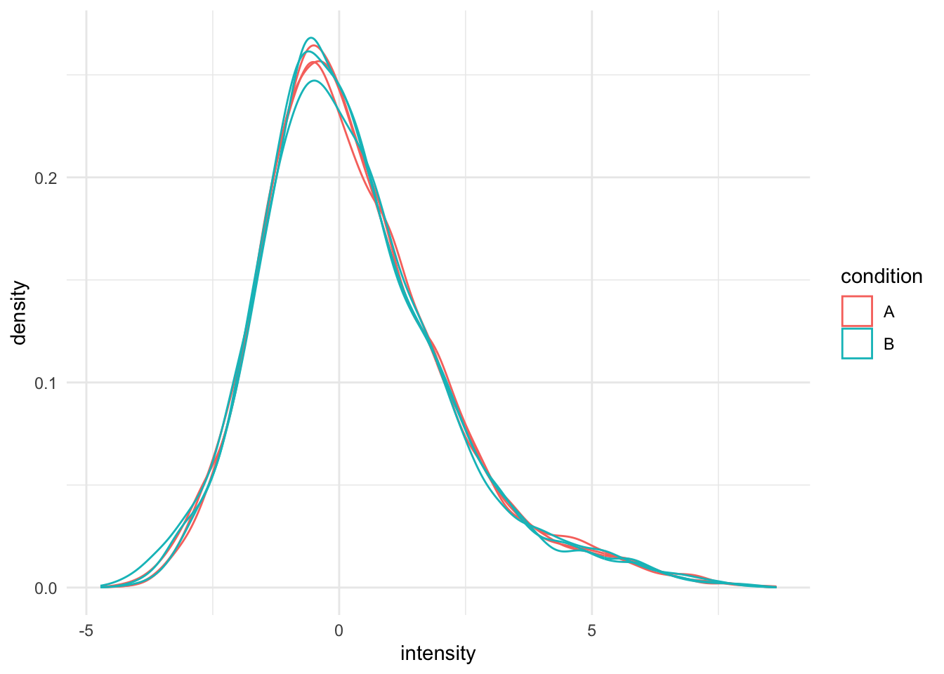

We can visualize our data using a Multi Dimensional Scaling plot, eg. as provided by the limma package.

pe[["peptideNorm"]] %>% 
  assay %>%
  limma::plotMDS(col = as.numeric(colData(pe)$condition))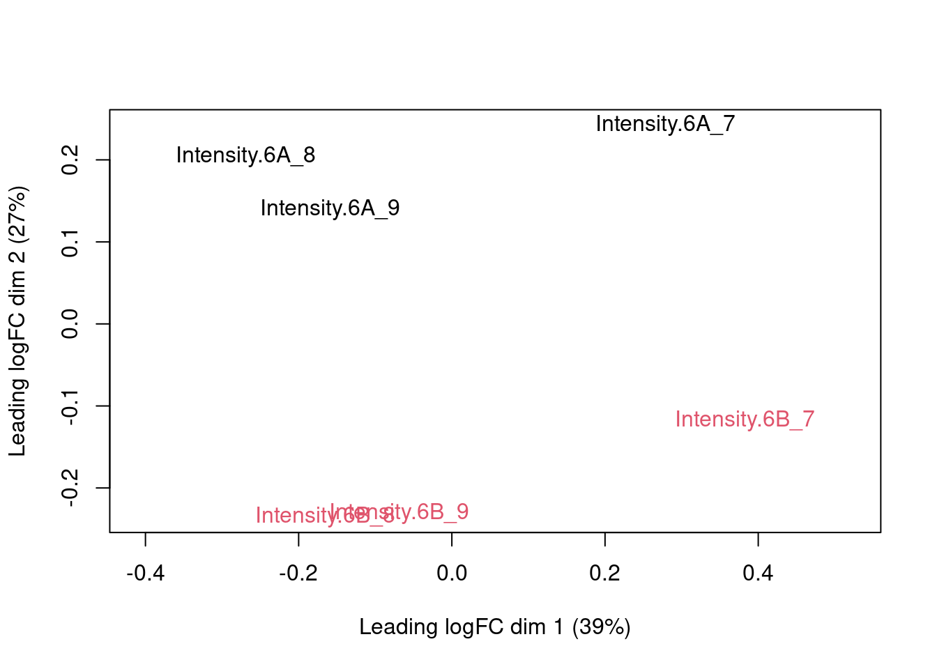

The first axis in the plot is showing the leading log fold changes (differences on the log scale) between the samples.

We notice that the leading differences (log FC) in the peptide data seems to be driven by technical variability. Indeed, the samples do not seem to be clearly separated according to the spike-in condition.

3.5 Summarization to protein level

• By default robust summarization is used: fun = MsCoreUtils::robustSummary()

pe <- aggregateFeatures(pe,
  i = "peptideNorm",
  fcol = "Proteins",
  na.rm = TRUE,
  name = "protein")

## Your quantitative and row data contain missing values. Please read the
## relevant section(s) in the aggregateFeatures manual page regarding the
## effects of missing values on data aggregation.

plotMDS(assay(pe[["protein"]]), col = as.numeric(colData(pe)$condition))

Note that the samples upon robust summarisation show a clear separation according to the spike-in condition in the second dimension of the MDS plot.

4 Data Analysis

4.1 Estimation

We model the protein level expression values using msqrob. By default msqrob2 estimates the model parameters using robust regression.

We will model the data with a different group mean. The group is incoded in the variable condition of the colData. We can specify this model by using a formula with the factor condition as its predictor: formula = ~condition.

Note, that a formula always starts with a symbol ‘~’.

pe <- msqrob(object = pe, i = "protein", formula = ~condition)

4.2 Inference

First, we extract the parameter names of the model by looking at the first model. The models are stored in the row data of the assay under the default name msqrobModels.

getCoef(rowData(pe[["protein"]])$msqrobModels[[1]])

## (Intercept)  conditionB 
##   -2.672396    1.513682

We can also explore the design of the model that we specified using the the package ExploreModelMatrix

library(ExploreModelMatrix)
VisualizeDesign(colData(pe),~condition)$plotlist[[1]]

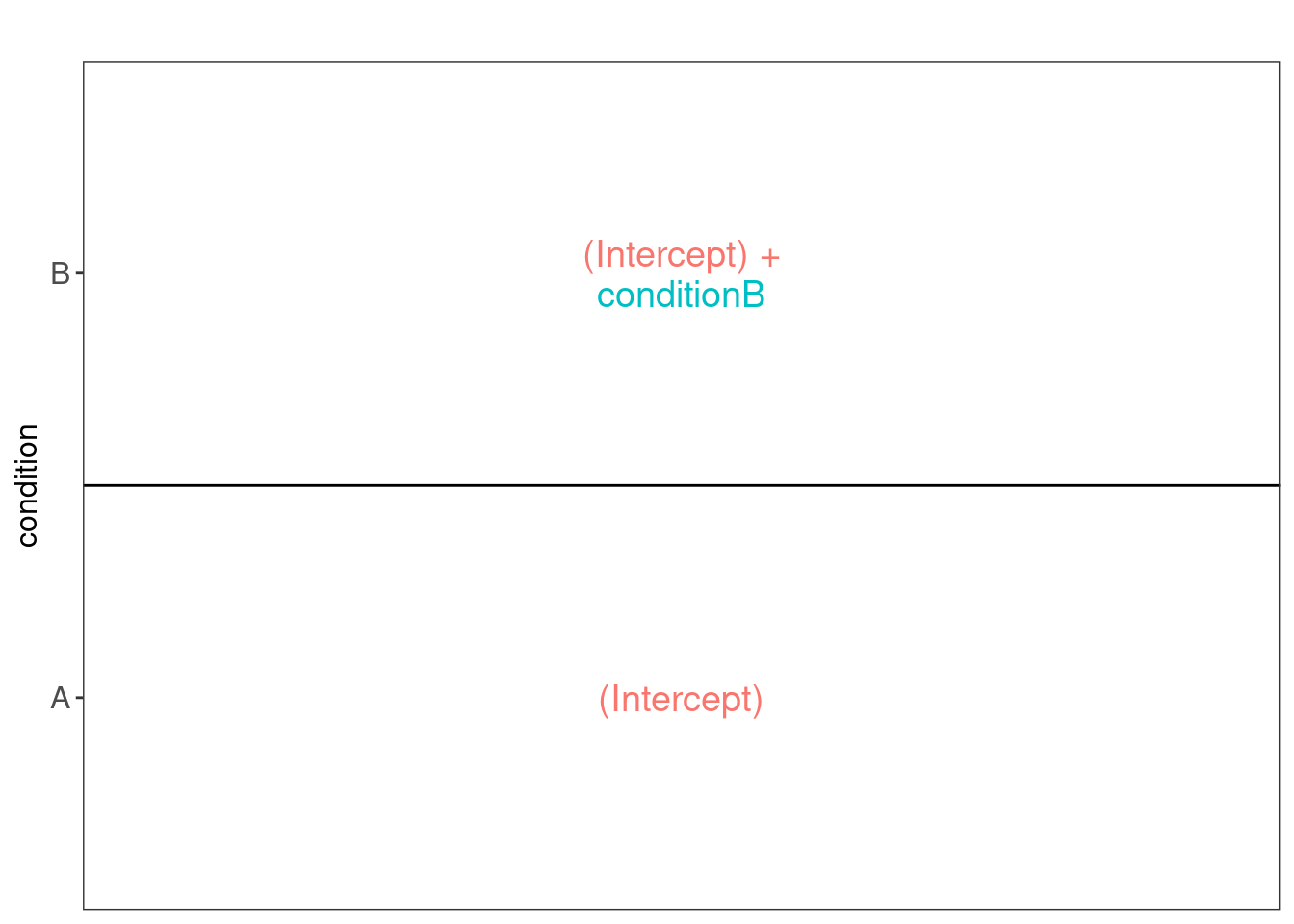
Spike-in condition A is the reference class. So the mean log2 expression for samples from condition A is ‘(Intercept). The mean log2 expression for samples from condition B is’(Intercept)+conditionB’. Hence, the average log2 fold change between condition b and condition a is modelled using the parameter ‘conditionB’. Thus, we assess the contrast ‘conditionB = 0’ with our statistical test.

L <- makeContrast("conditionB=0", parameterNames = c("conditionB"))
pe <- hypothesisTest(object = pe, i = "protein", contrast = L)

4.3 Plots

4.3.1 Volcano-plot

volcano <- ggplot(rowData(pe[["protein"]])$conditionB,
                  aes(x = logFC, y = -log10(pval), color = adjPval < 0.05)) +
  geom_point(cex = 2.5) +
  scale_color_manual(values = alpha(c("black", "red"), 0.5)) + theme_minimal()
volcano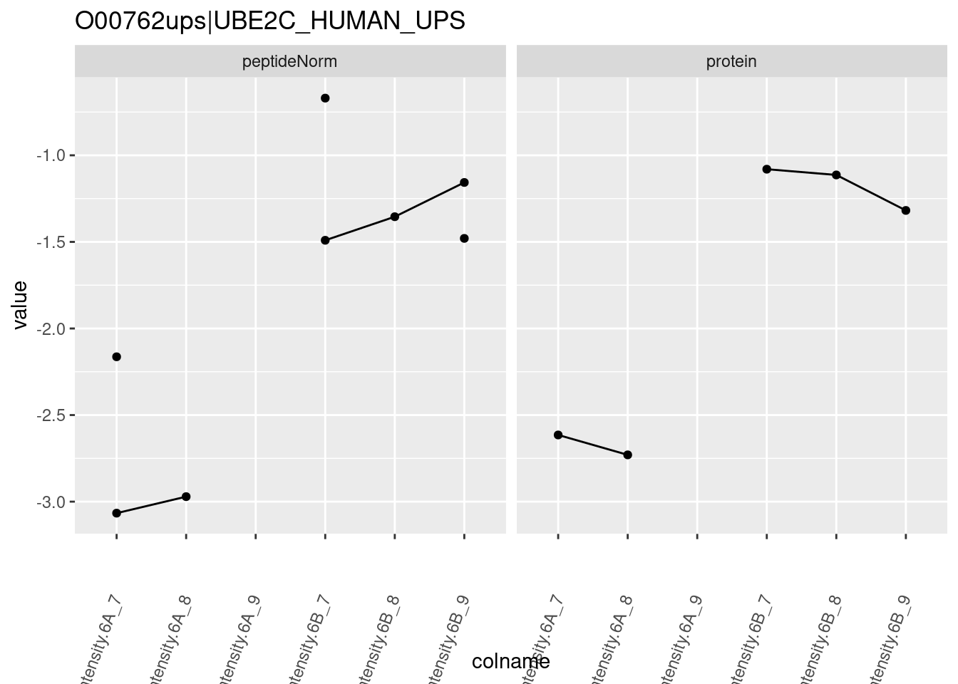

Note, that 20 proteins are found to be differentially abundant.

4.3.2 Heatmap

We first select the names of the proteins that were declared signficant.

sigNames <- rowData(pe[["protein"]])$conditionB %>%
  rownames_to_column("protein") %>%
  filter(adjPval<0.05) %>%
  pull(protein)
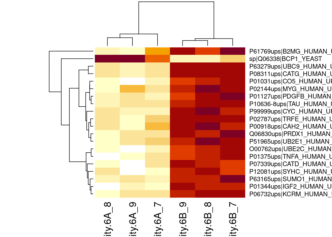
heatmap(assay(pe[["protein"]])[sigNames, ])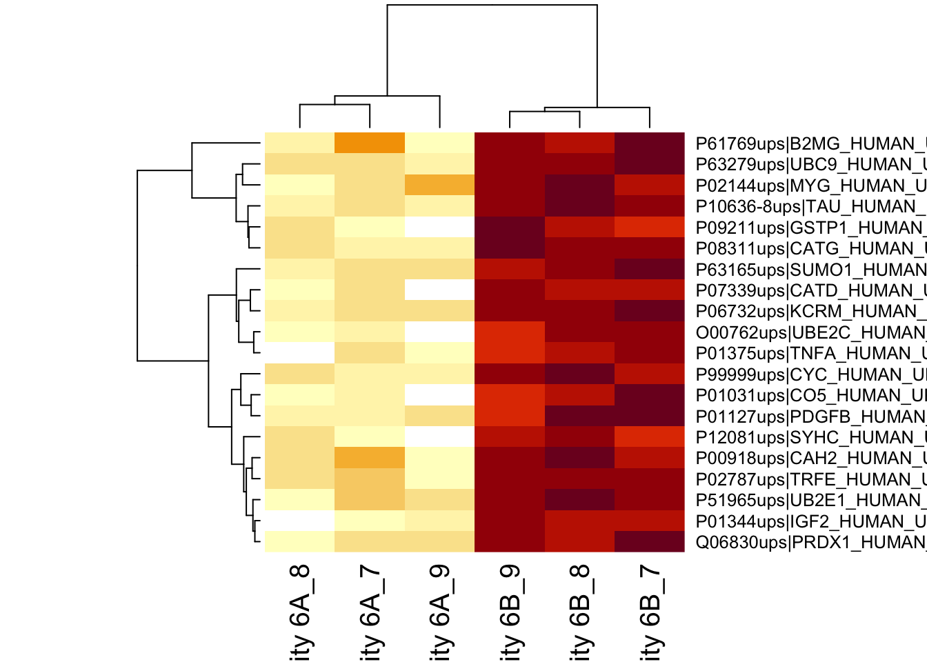

The majority of the proteins are indeed UPS proteins. 1 yeast protein is returned. Note, that the yeast protein indeed shows evidence for differential abundance.

4.3.3 Boxplots

We make boxplot of the log2 FC and stratify according to the whether a protein is spiked or not.

rowData(pe[["protein"]])$conditionB %>%
  rownames_to_column(var = "protein") %>%
  ggplot(aes(x=grepl("UPS",protein),y=logFC)) +
  geom_boxplot() +
  xlab("UPS") +
  geom_segment(
    x = 1.5,
    xend = 2.5,
    y = log2(0.74/0.25),
    yend = log2(0.74/0.25),
    colour="red") +
  geom_segment(
    x = 0.5,
    xend = 1.5,
    y = 0,
    yend = 0,
    colour="red") +
  annotate(
    "text",
    x = c(1,2),
    y = c(0,log2(0.74/0.25))+.1,
    label = c(
      "log2 FC Ecoli = 0",
      paste0("log2 FC UPS = ",round(log2(0.74/0.25),2))
      ),
    colour = "red")

## Warning: Removed 167 rows containing non-finite values (stat_boxplot).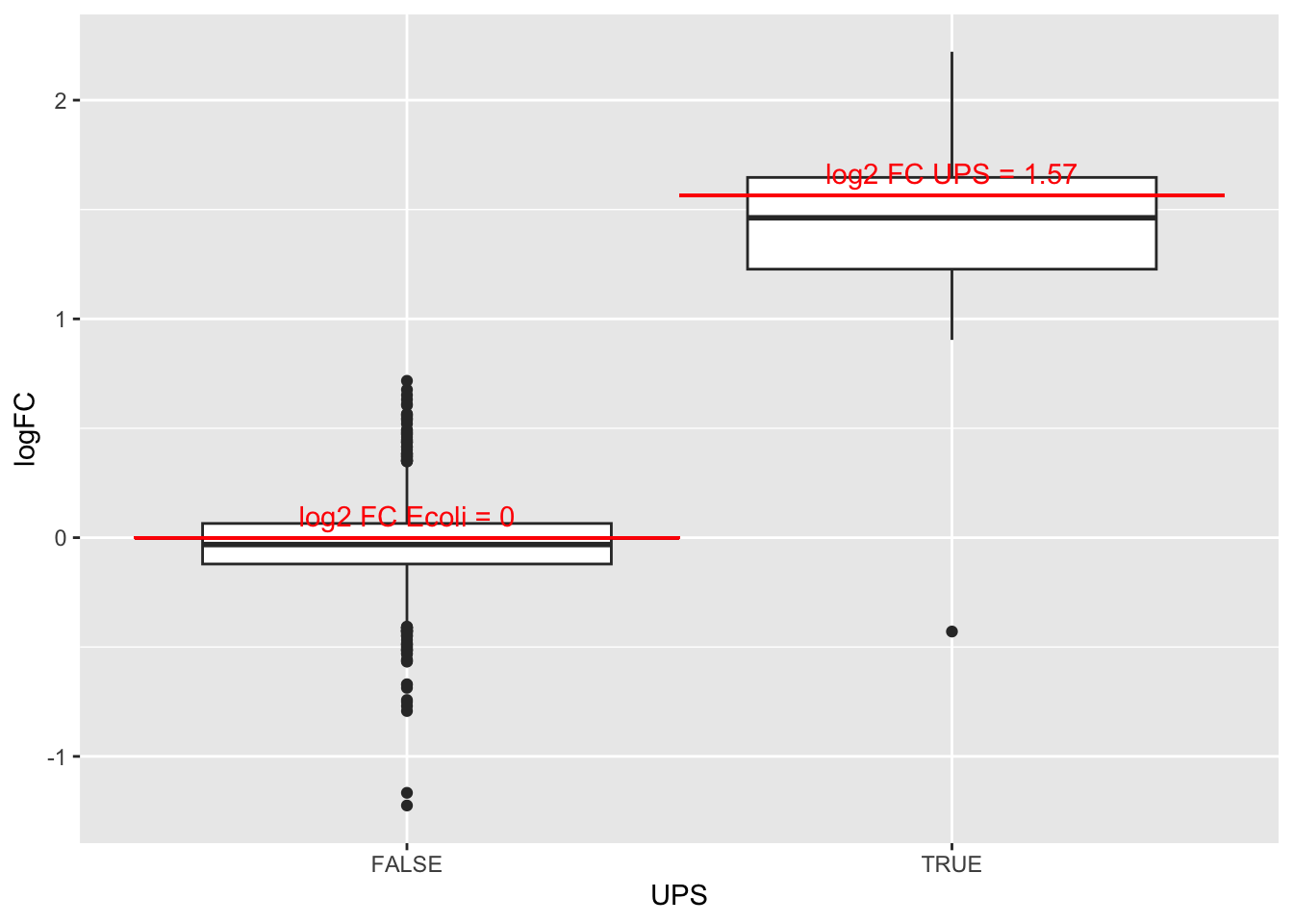

What do you observe?

4.3.4 Detail plots

We first extract the normalized peptideRaw expression values for a particular protein.

for (protName in sigNames)
{
pePlot <- pe[protName, , c("peptideNorm","protein")]
pePlotDf <- data.frame(longFormat(pePlot))
pePlotDf$assay <- factor(pePlotDf$assay,
                        levels = c("peptideNorm", "protein"))
pePlotDf$condition <- as.factor(colData(pePlot)[pePlotDf$colname, "condition"])

# plotting
p1 <- ggplot(data = pePlotDf,
       aes(x = colname, y = value, group = rowname)) +
    geom_line() + 
    geom_point() +  
    theme(axis.text.x = element_text(angle = 70, hjust = 1, vjust = 0.5)) +
    facet_grid(~assay) + 
    ggtitle(protName)
print(p1)

# plotting 2
p2 <- ggplot(pePlotDf, aes(x = colname, y = value, fill = condition)) +
  geom_boxplot(outlier.shape = NA) + 
  geom_point(
    position = position_jitter(width = .1),
    aes(shape = rowname)) +
  scale_shape_manual(values = 1:nrow(pePlotDf)) +
  labs(title = protName, x = "sample", y = "peptide intensity (log2)") + 
  theme(axis.text.x = element_text(angle = 70, hjust = 1, vjust = 0.5)) +
  facet_grid(~assay)
print(p2)
}

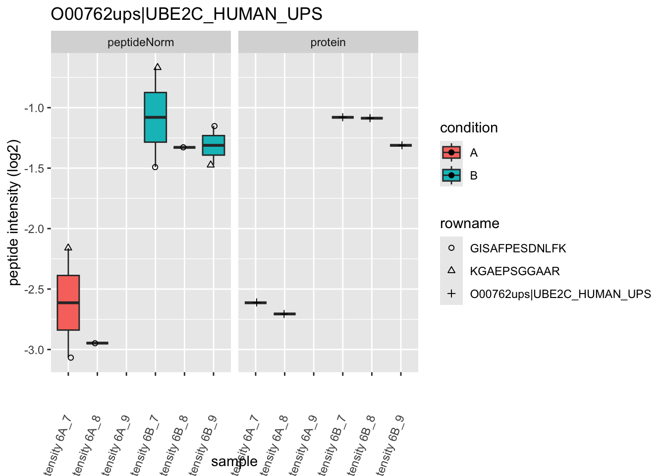
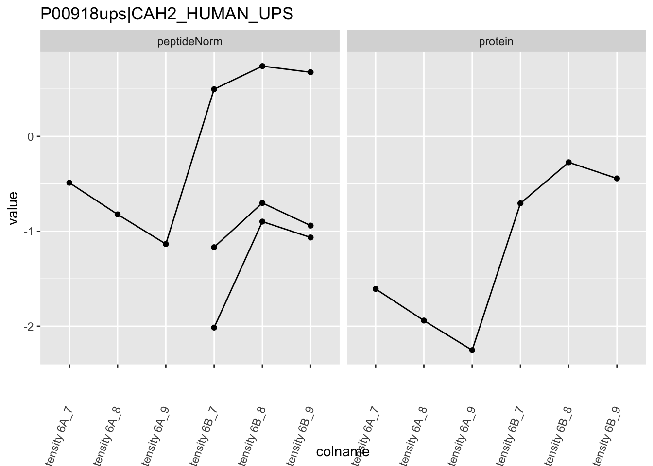
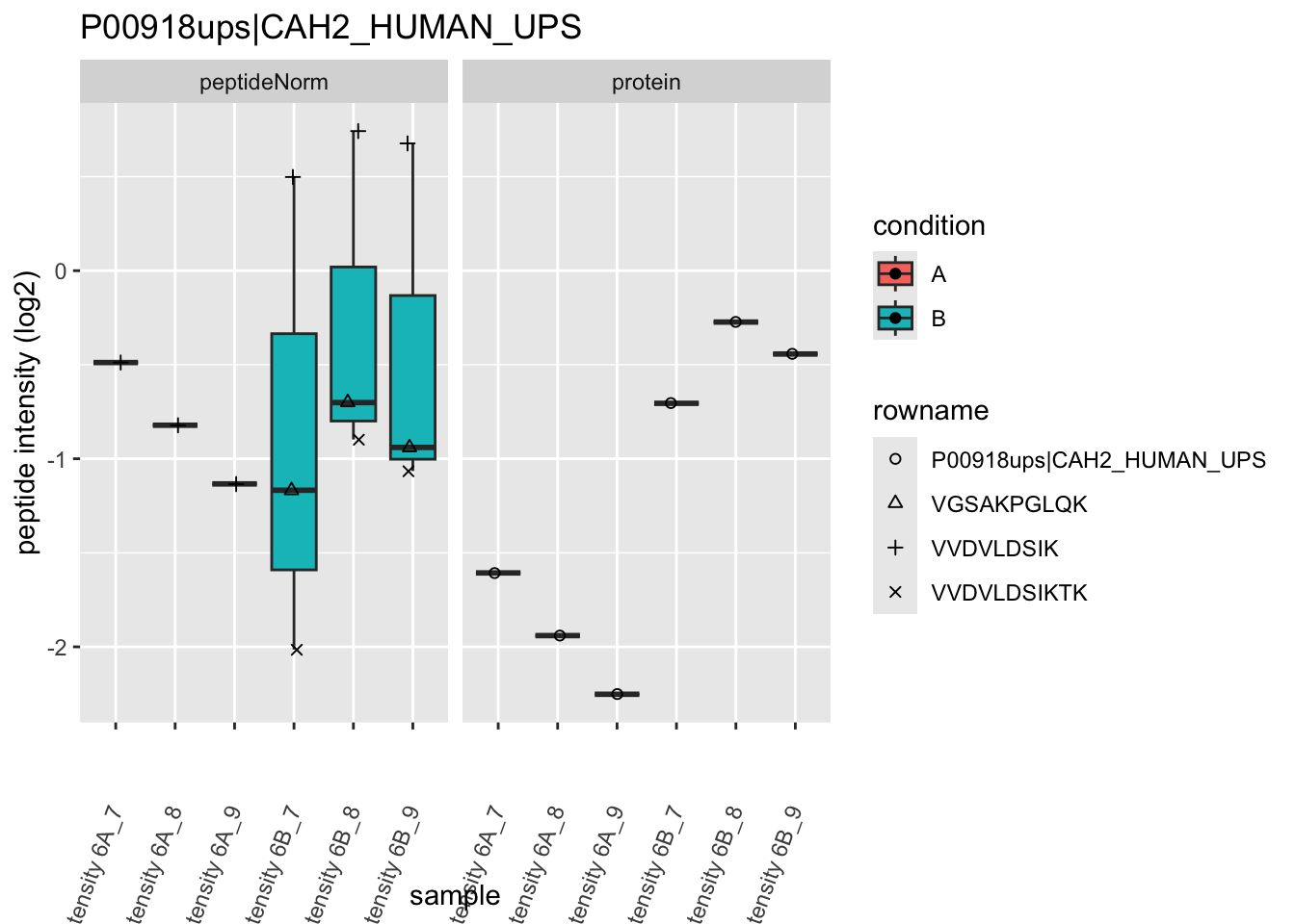
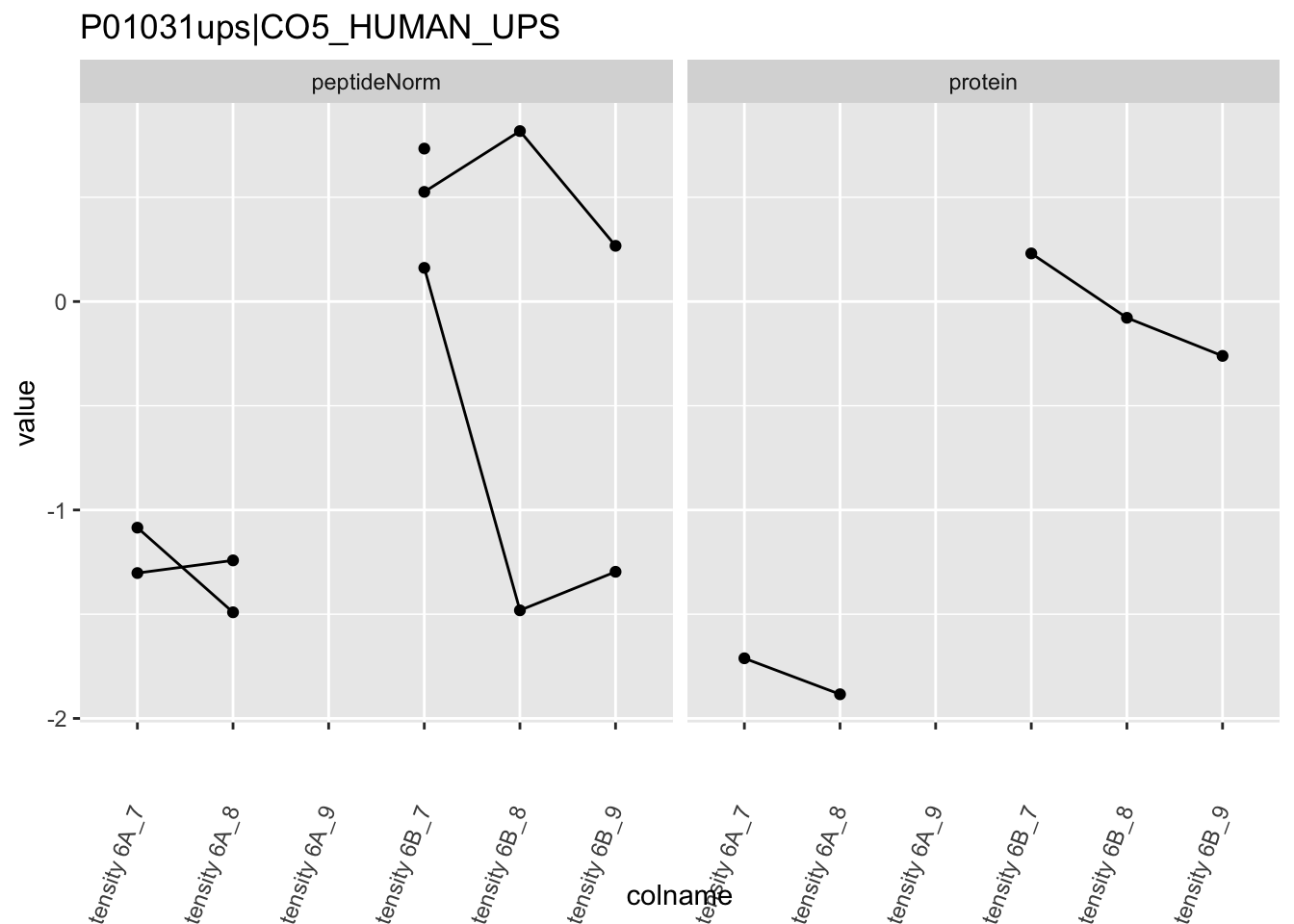
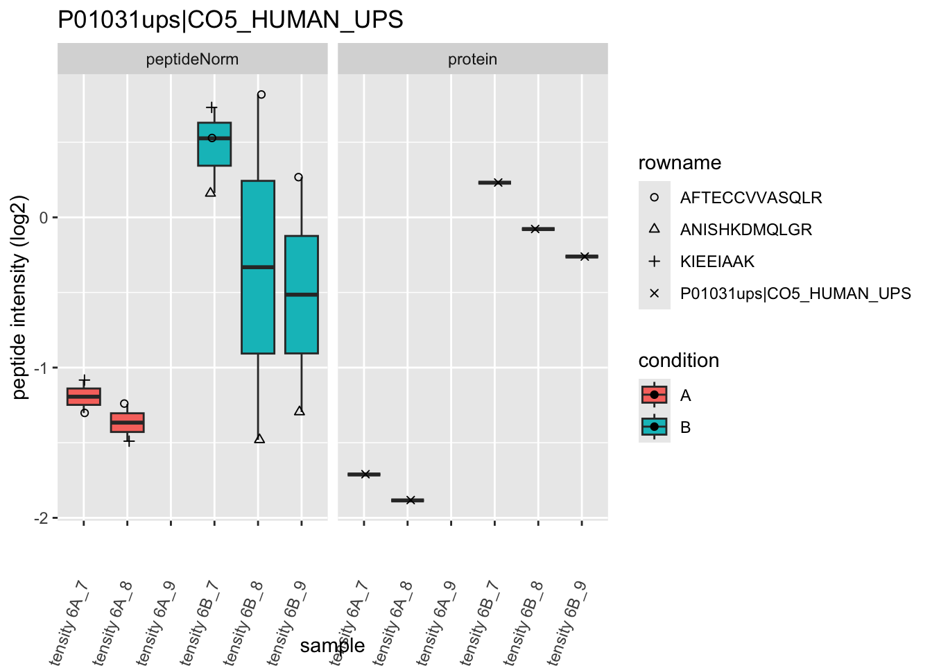
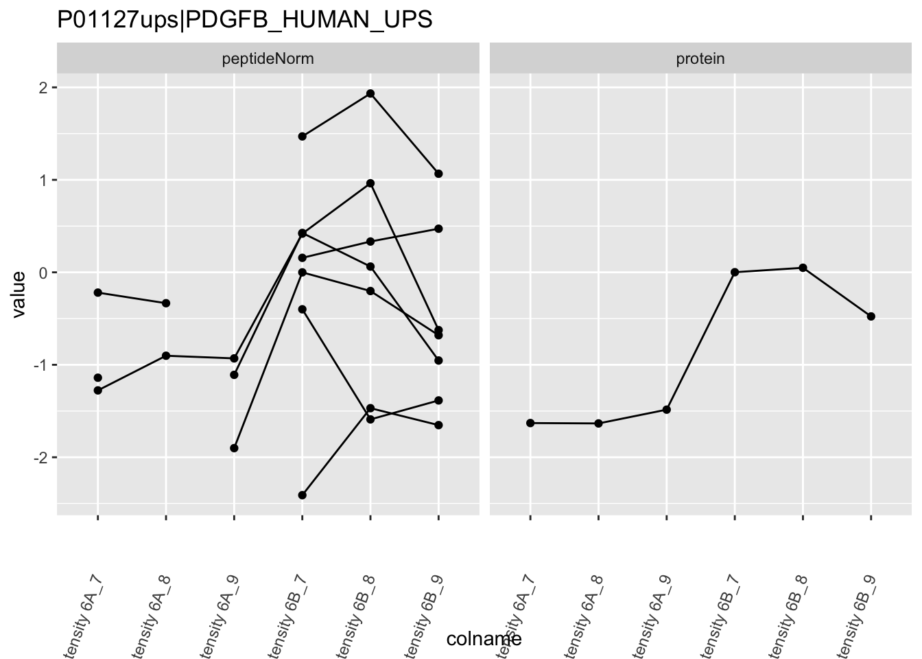
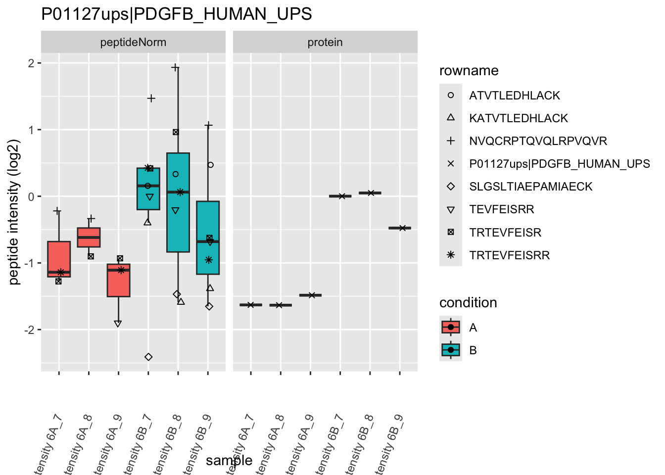
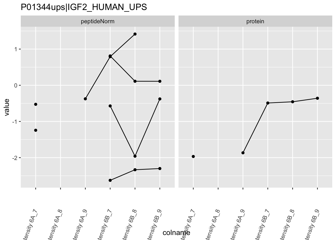
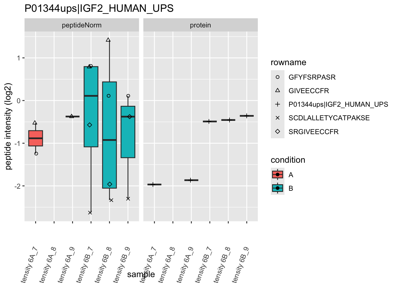
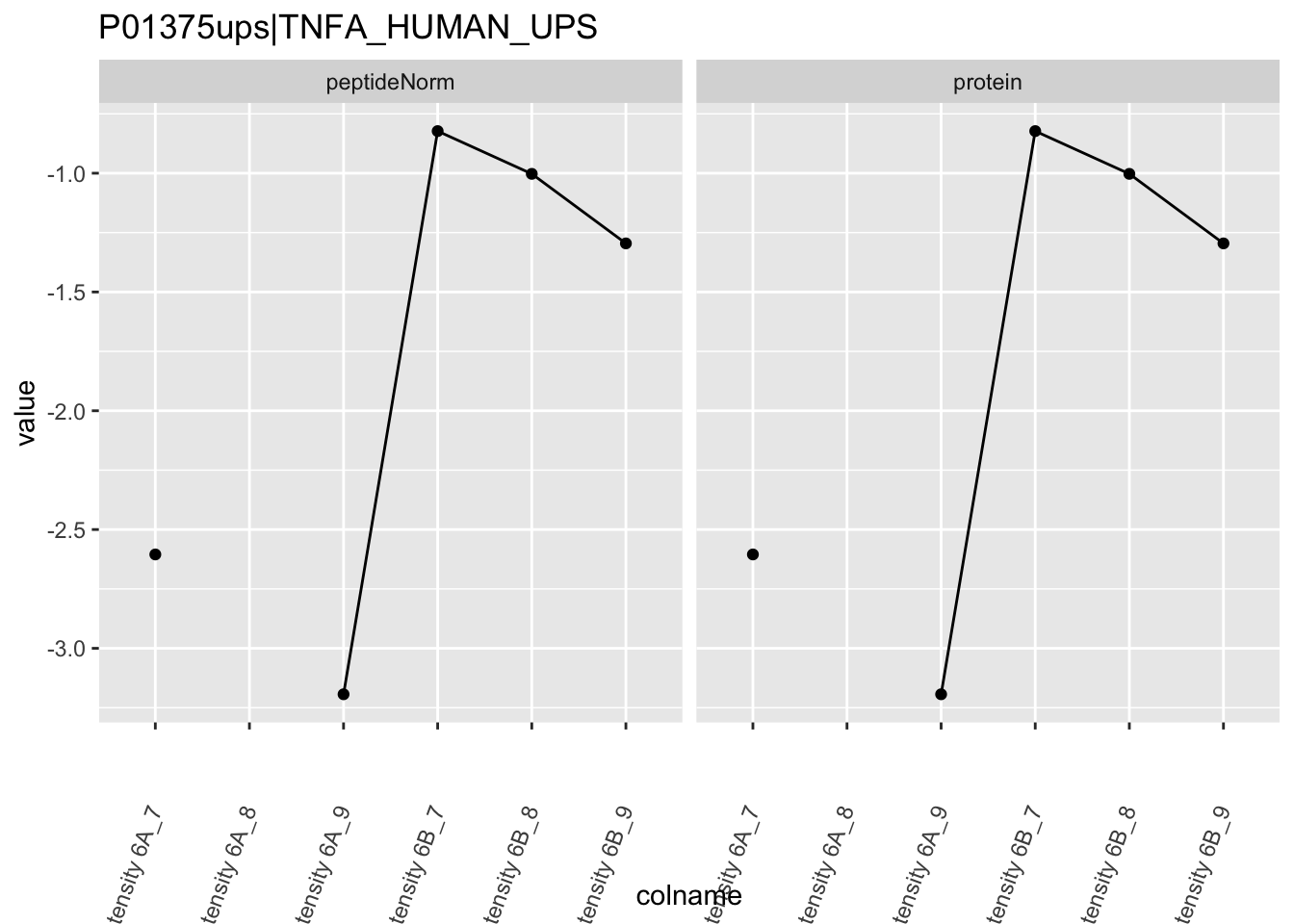
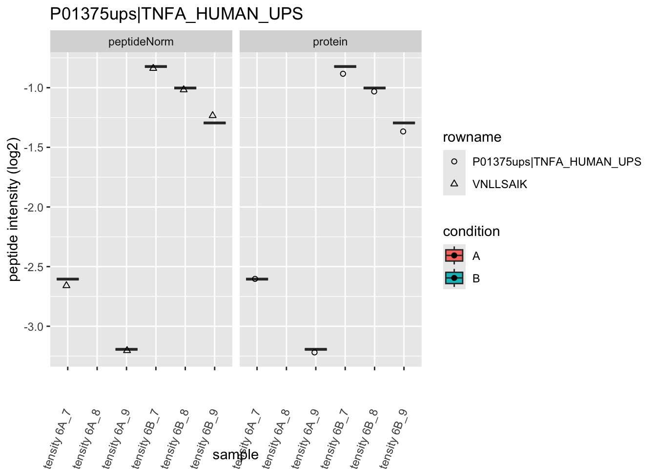
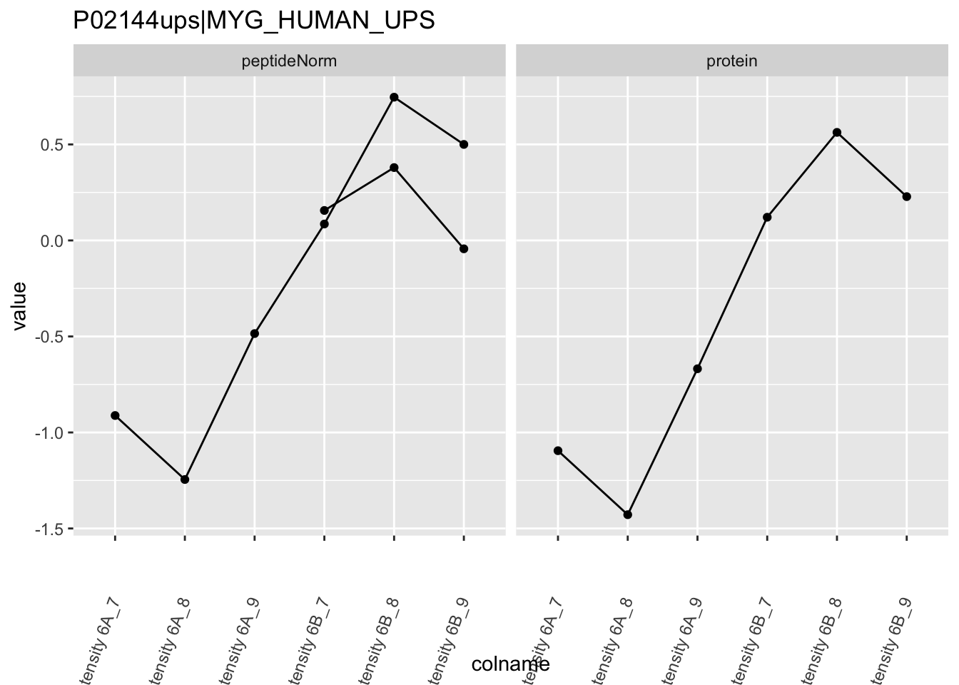
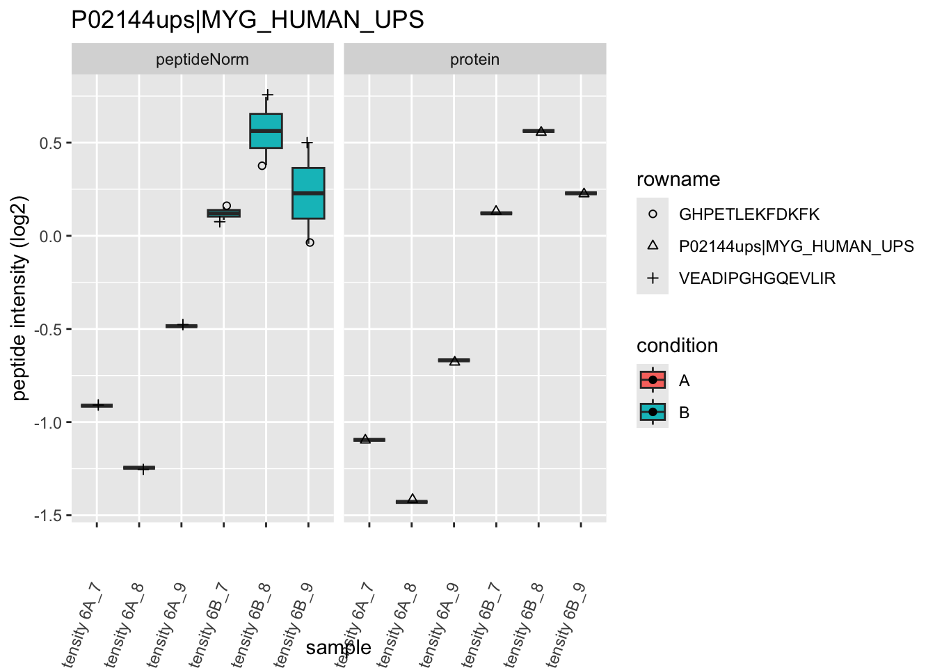
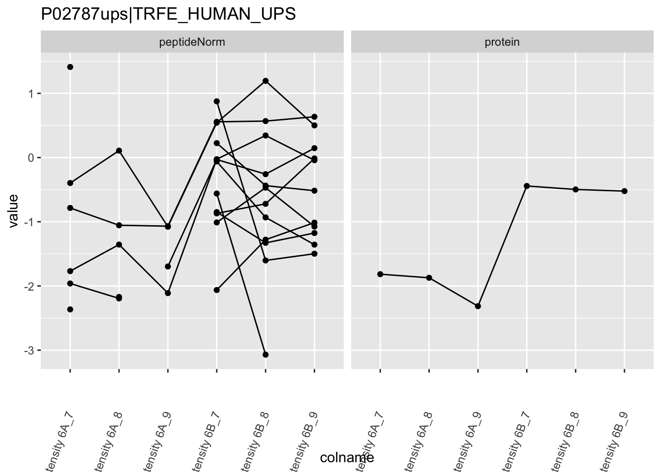
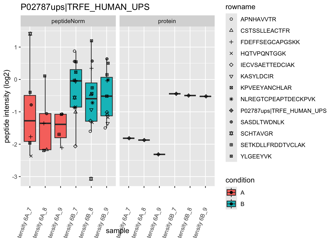
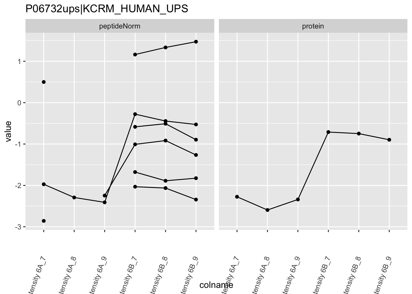
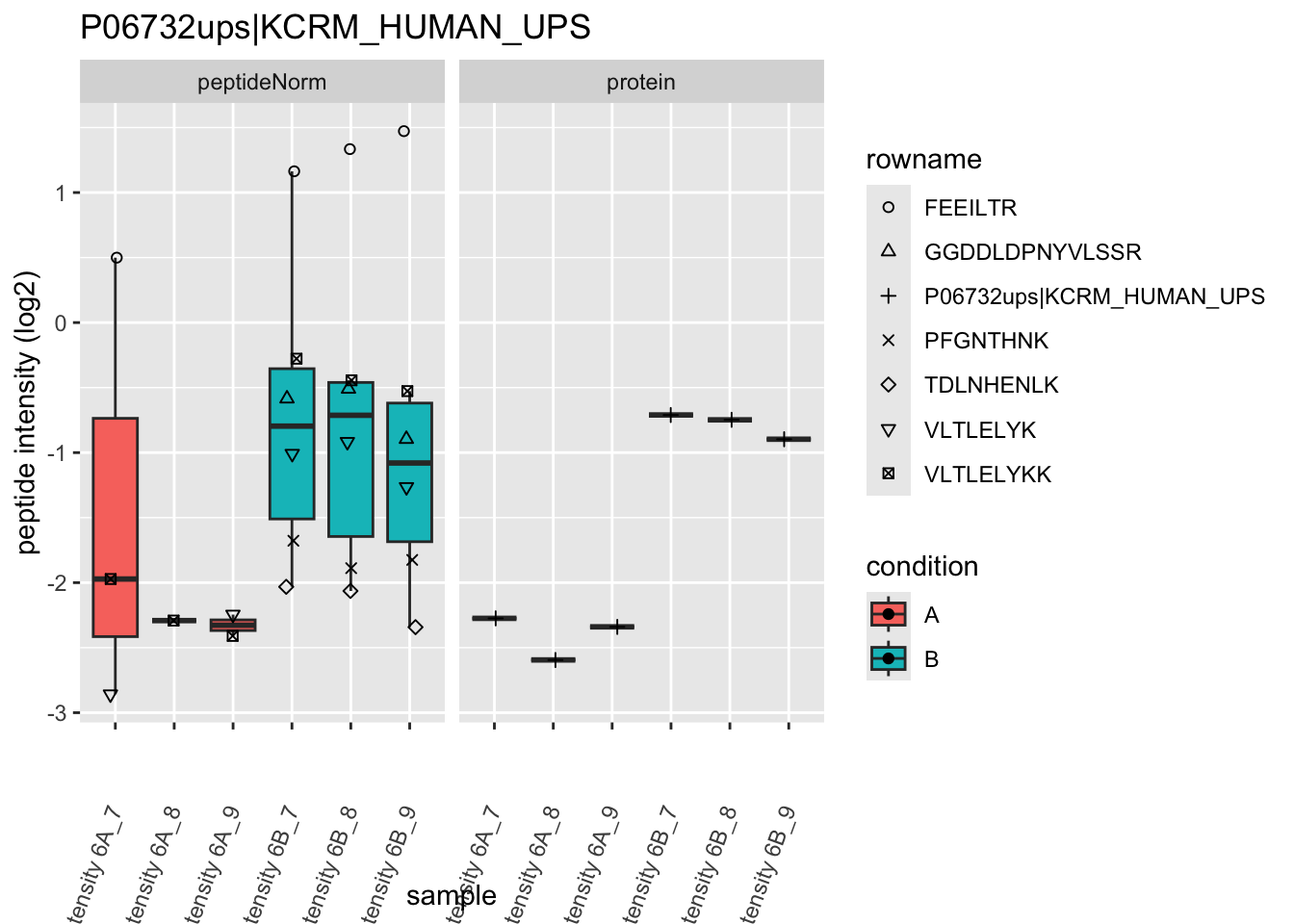
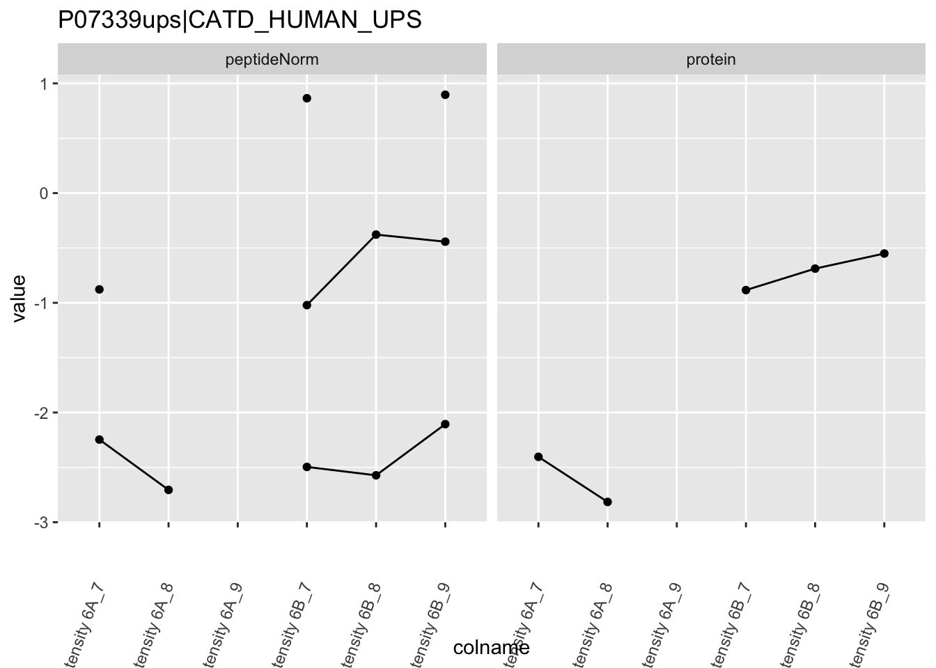
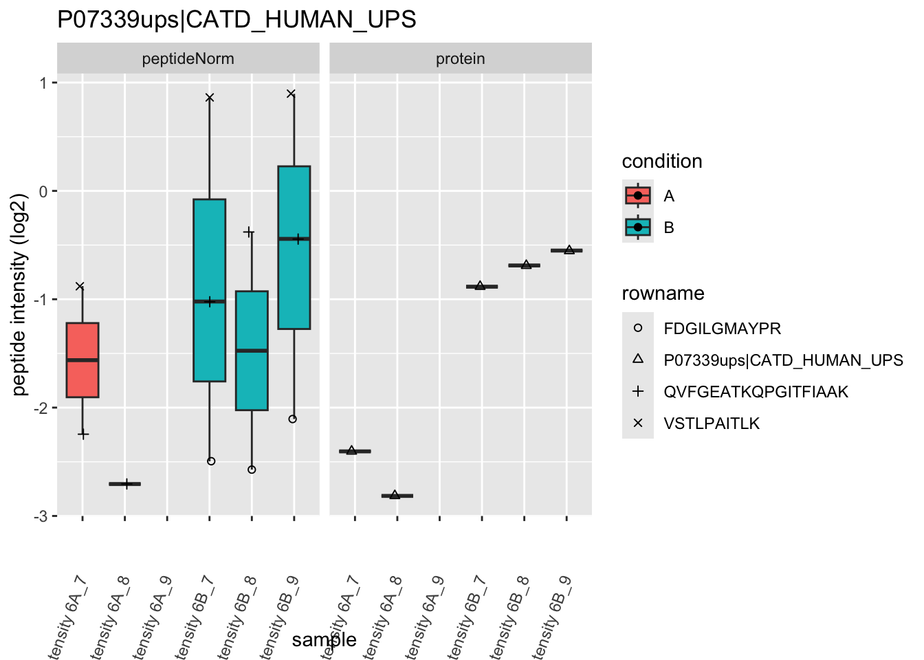
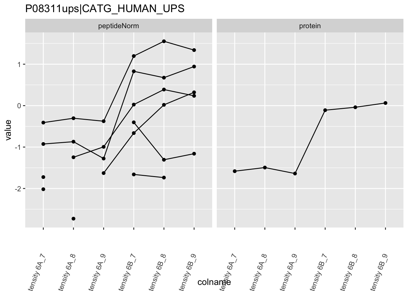
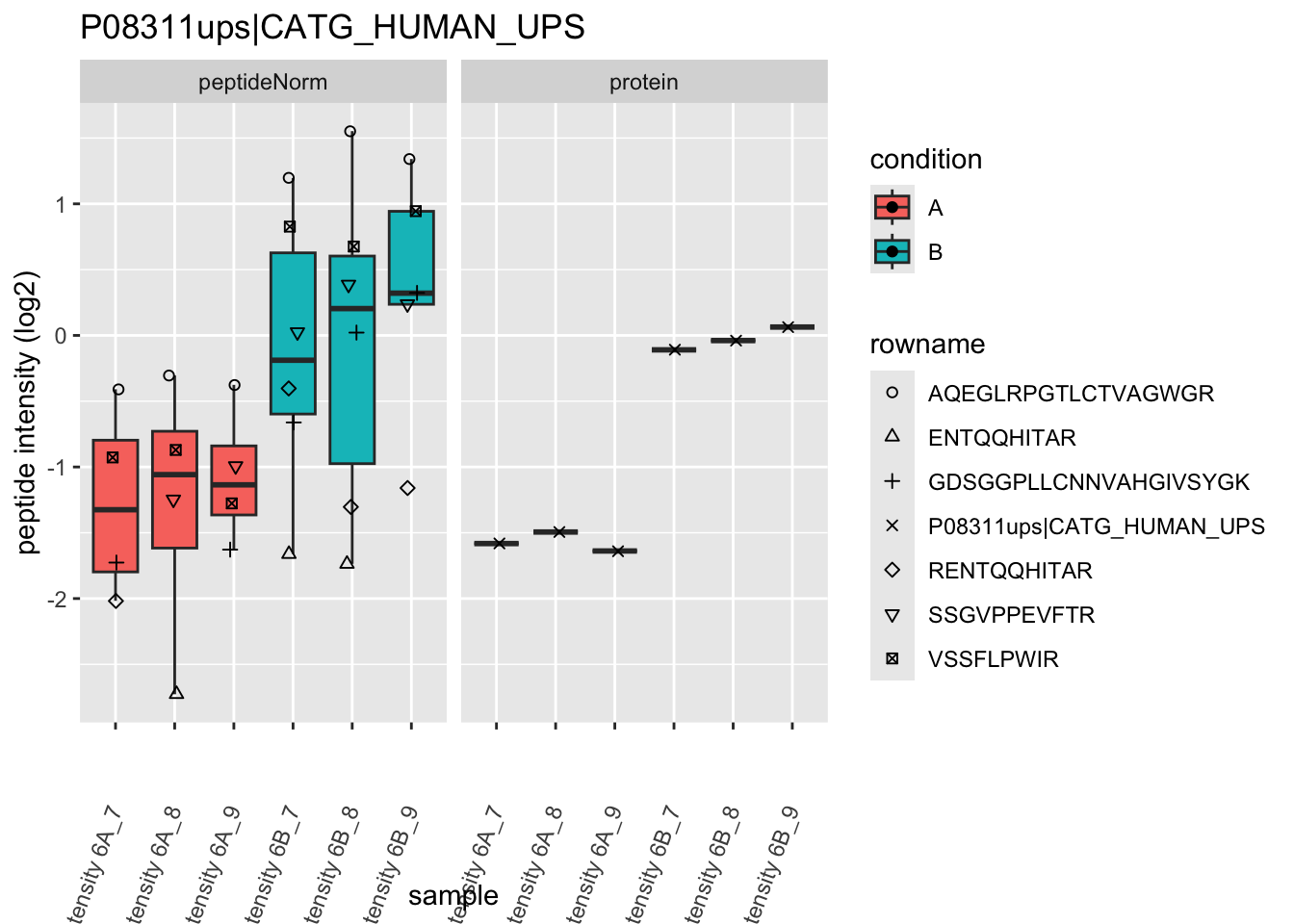
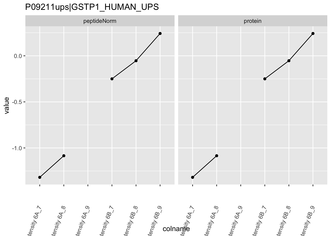
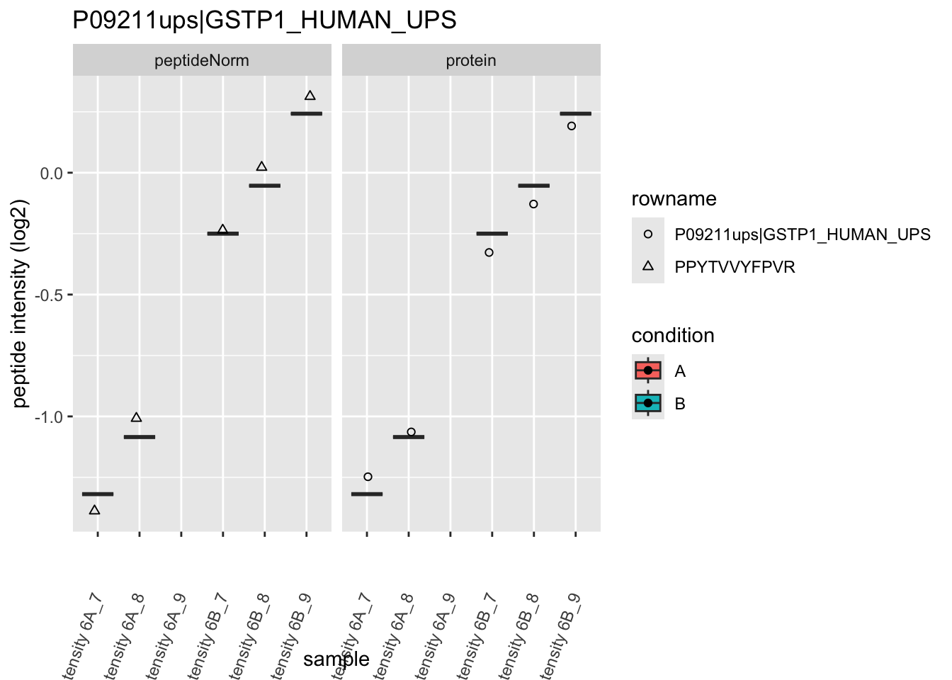
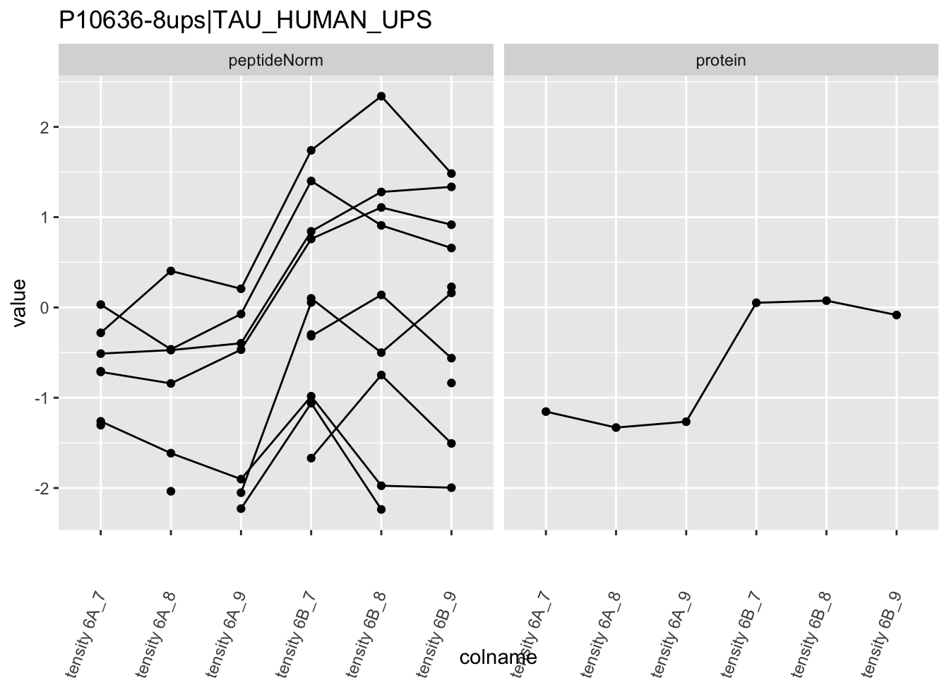
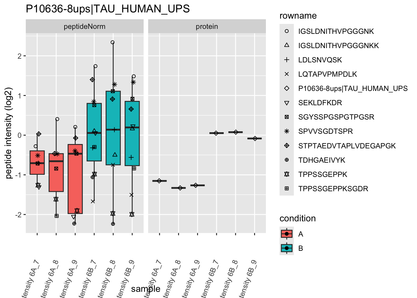
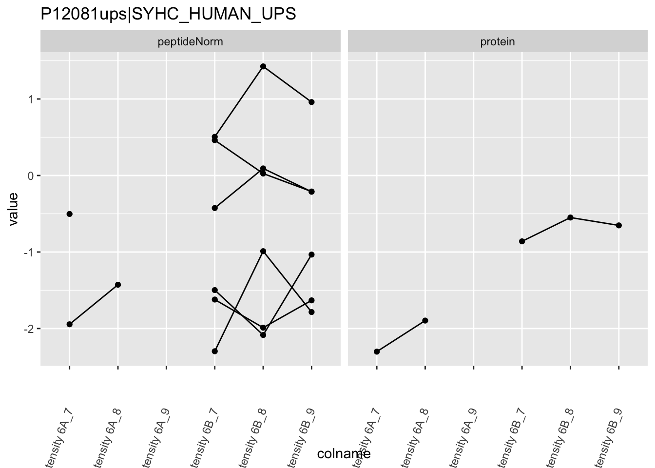
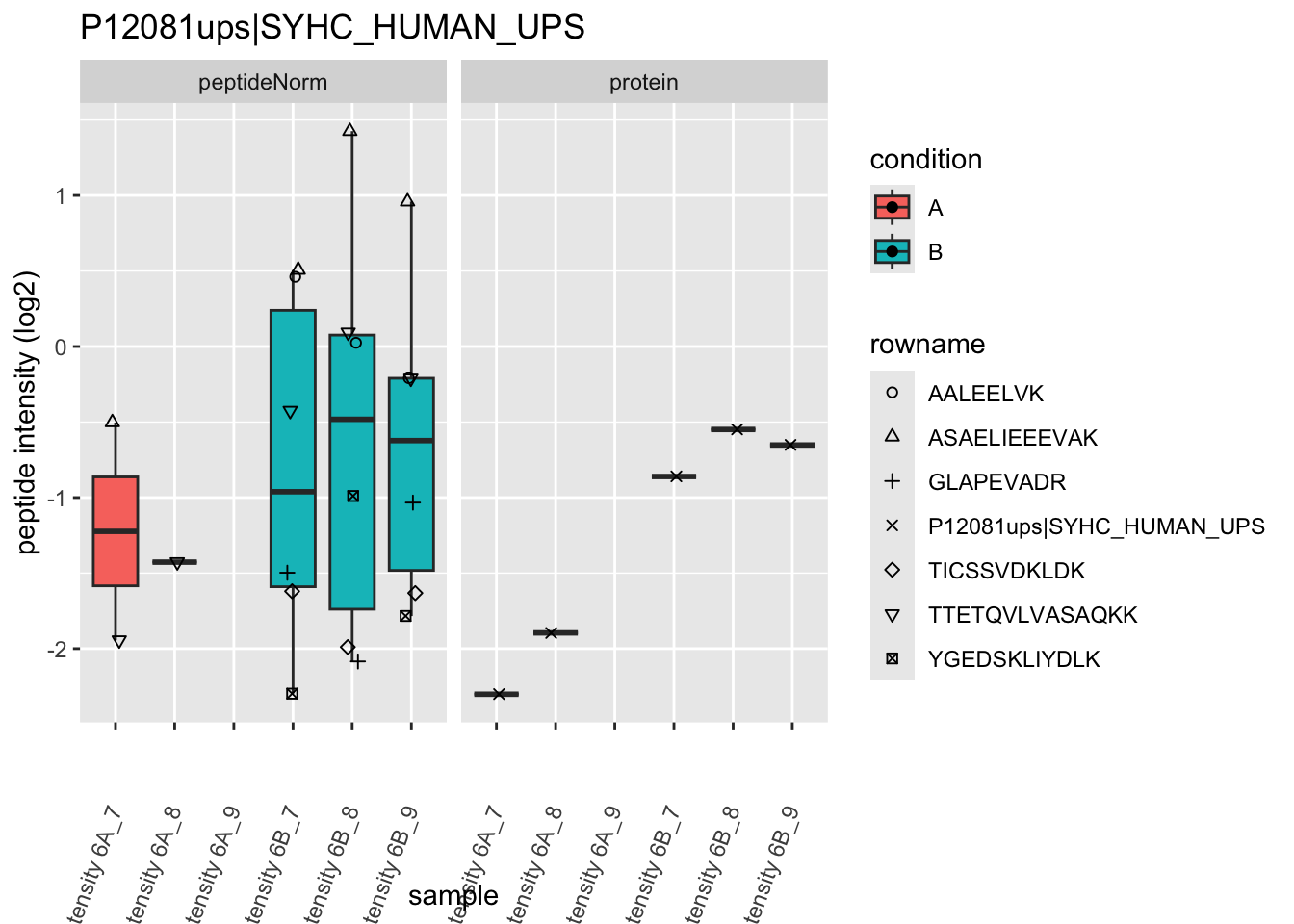
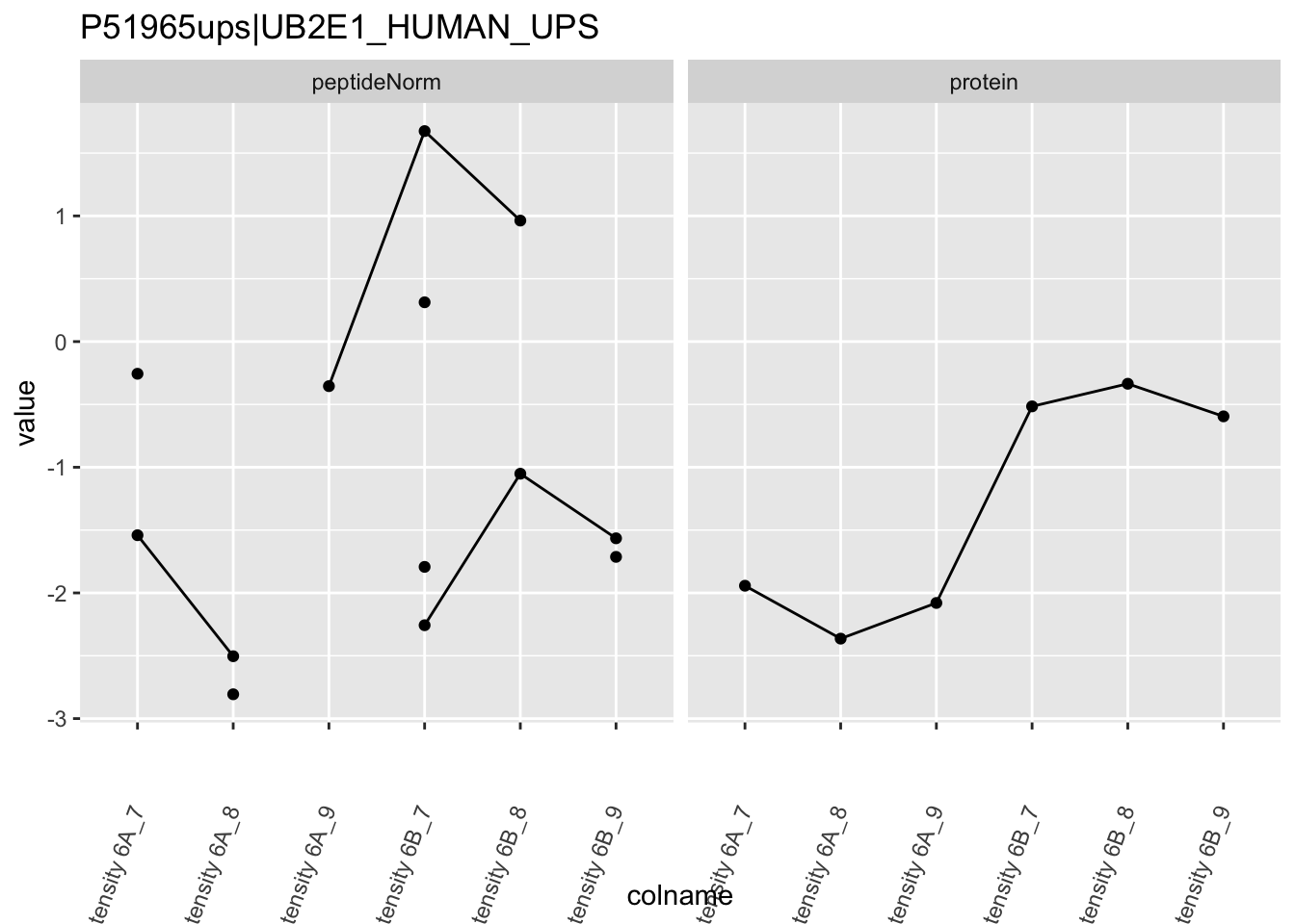
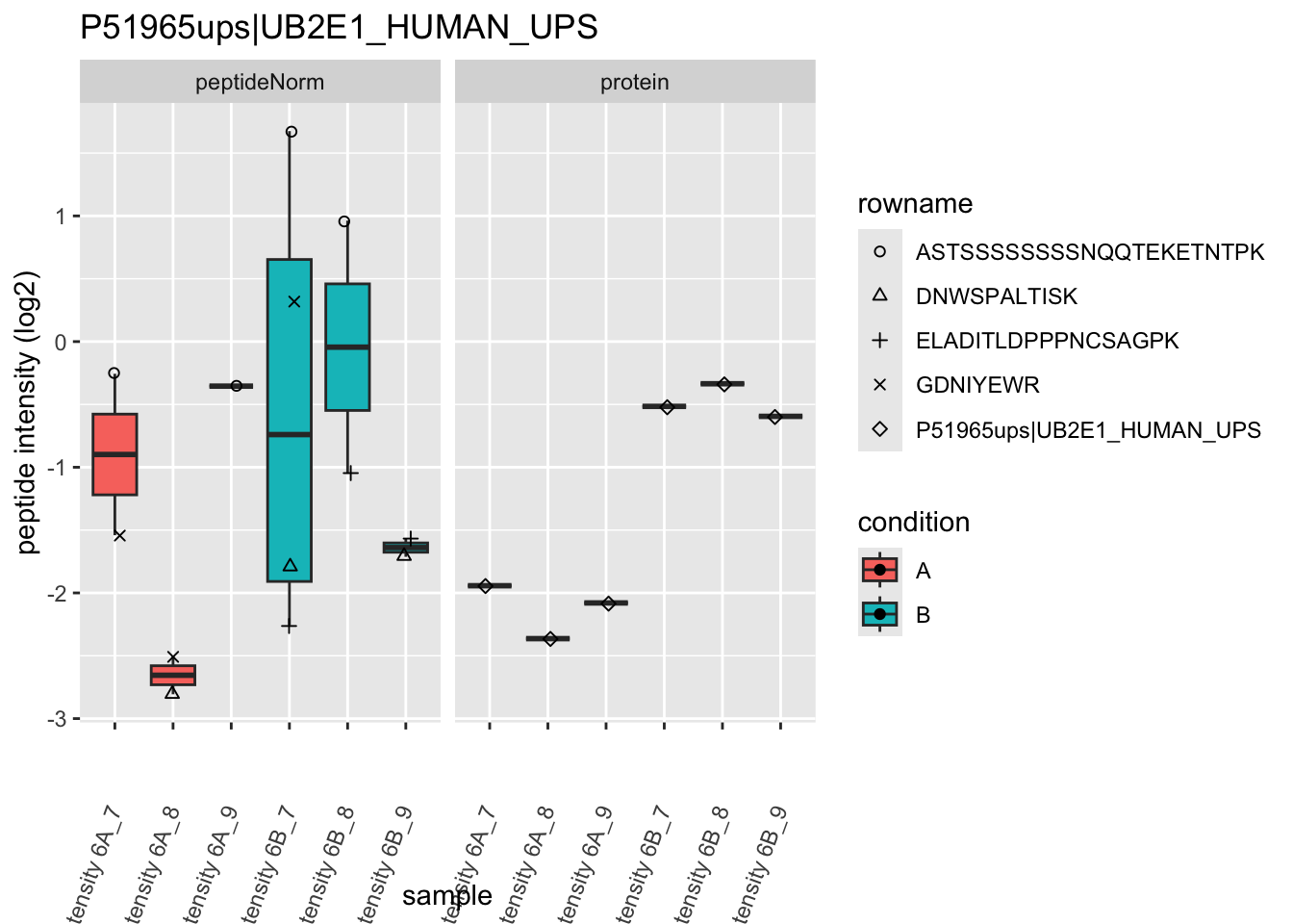
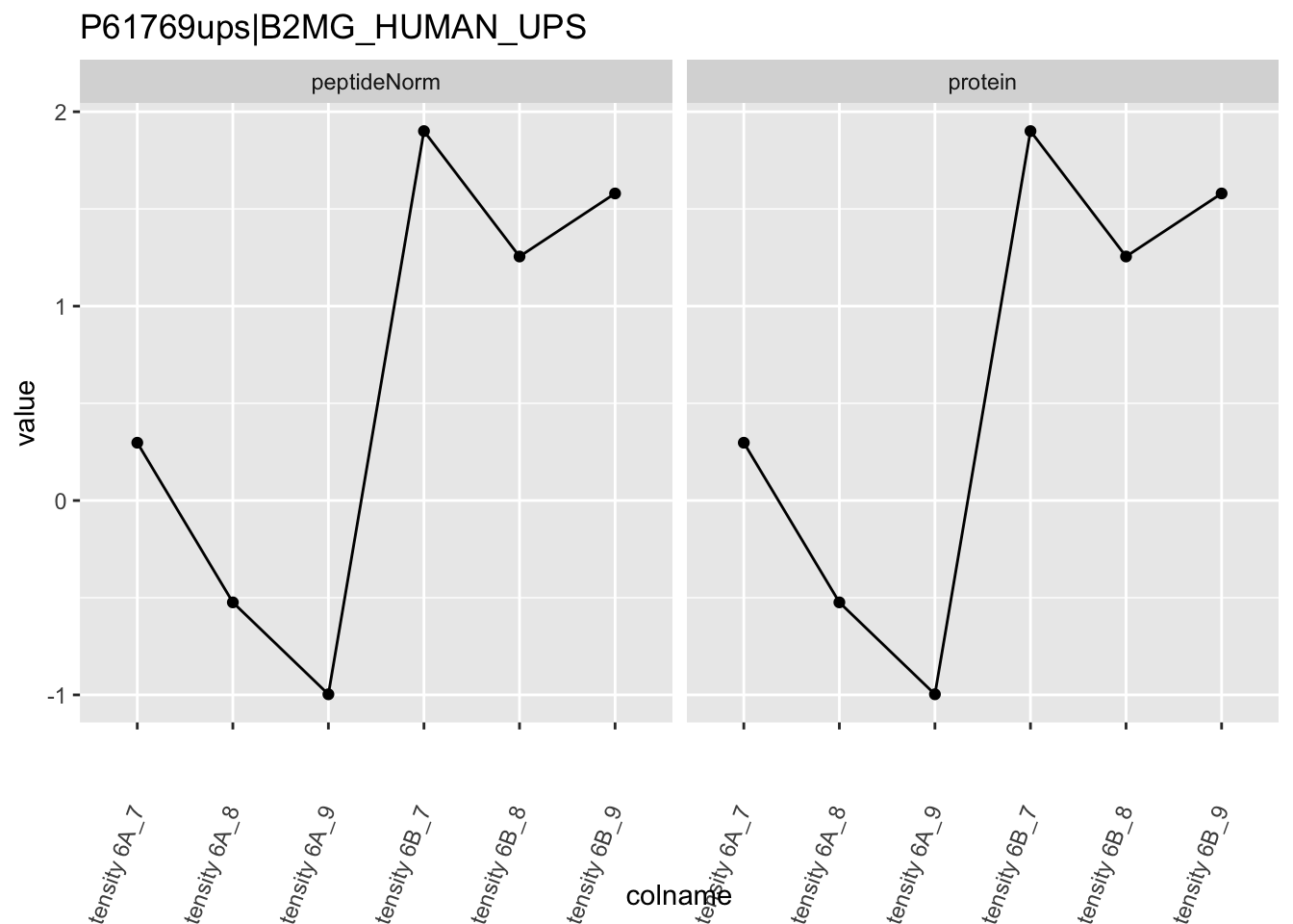
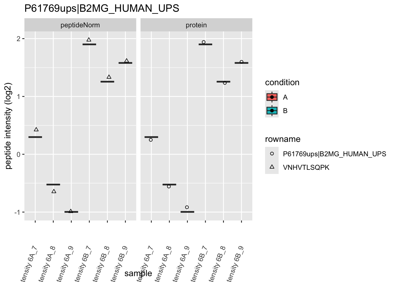
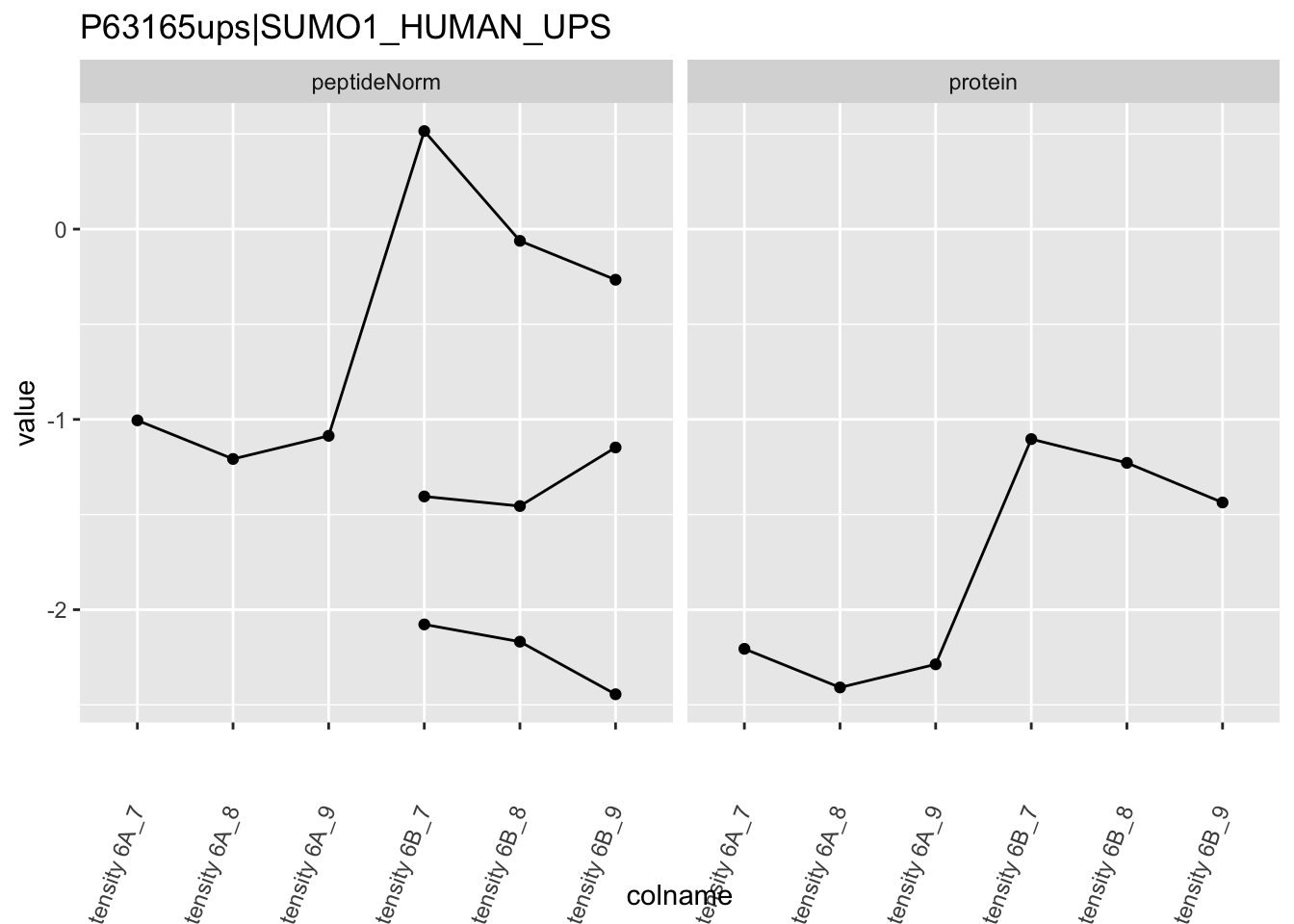
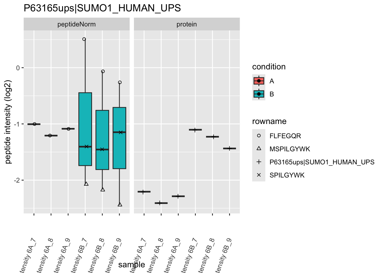
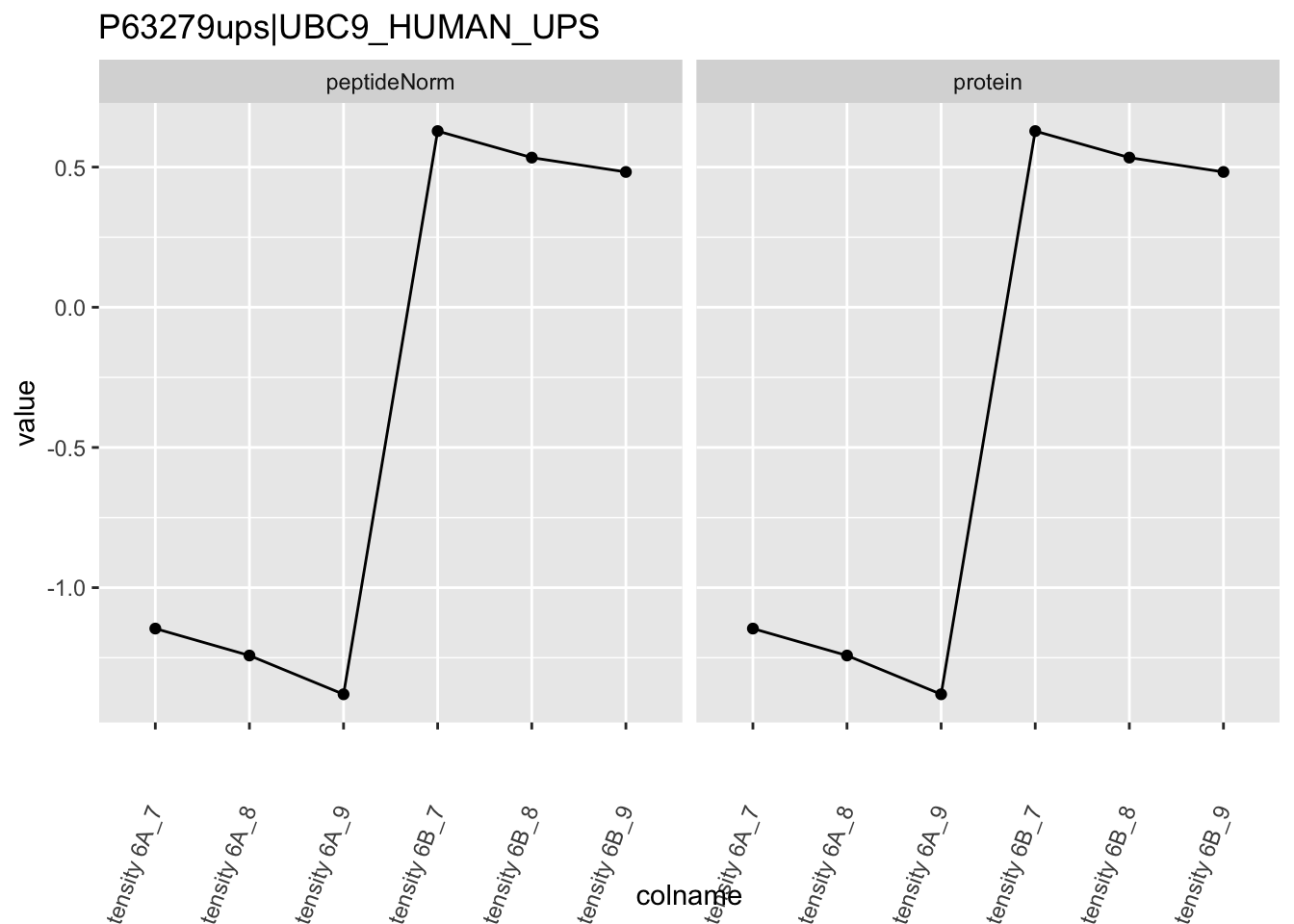
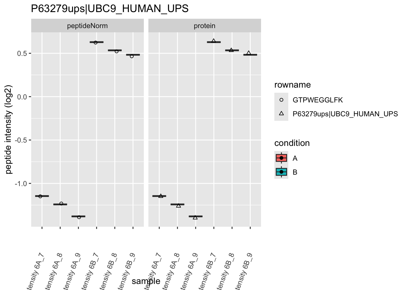
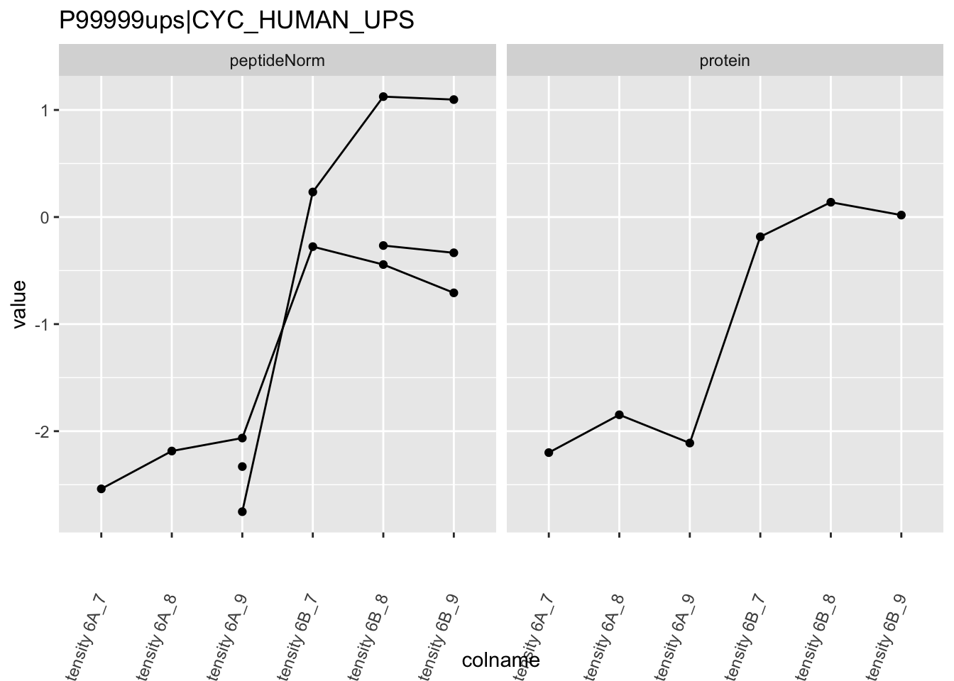
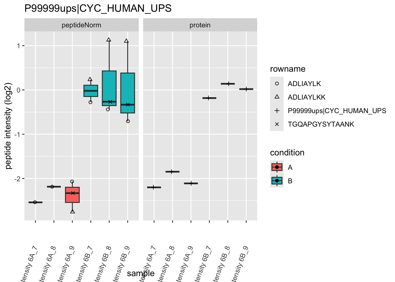
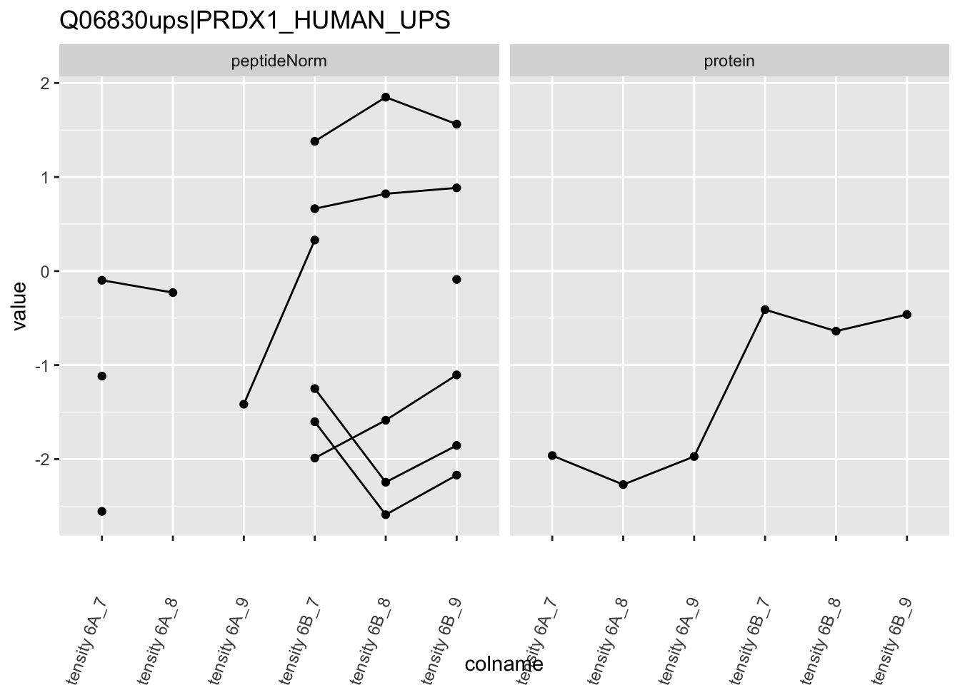
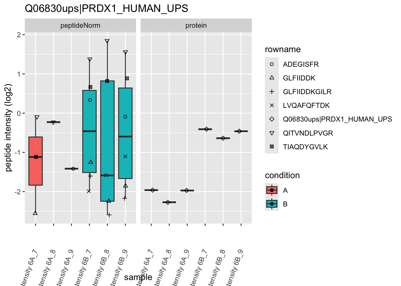
Note, that the yeast protein is only covered by 3 peptides. Only one peptide is picked up in condition A. This peptide is also only once observed in spike-in condition B. This puts a considerable burden upon the inference and could be avoided by more stringent filtering.

5 Session Info

With respect to reproducibility, it is highly recommended to include a session info in your script so that readers of your output can see your particular setup of R.

sessionInfo()

## R version 4.1.3 (2022-03-10)
## Platform: x86_64-pc-linux-gnu (64-bit)
## Running under: Ubuntu 22.04.2 LTS
## 
## Matrix products: default
## BLAS:   /usr/lib/x86_64-linux-gnu/openblas-pthread/libblas.so.3
## LAPACK: /usr/lib/x86_64-linux-gnu/openblas-pthread/libopenblasp-r0.3.20.so
## 
## locale:
##  [1] LC_CTYPE=C.UTF-8       LC_NUMERIC=C           LC_TIME=C.UTF-8       
##  [4] LC_COLLATE=C.UTF-8     LC_MONETARY=C.UTF-8    LC_MESSAGES=C.UTF-8   
##  [7] LC_PAPER=C.UTF-8       LC_NAME=C              LC_ADDRESS=C          
## [10] LC_TELEPHONE=C         LC_MEASUREMENT=C.UTF-8 LC_IDENTIFICATION=C   
## 
## attached base packages:
## [1] parallel  stats4    stats     graphics  grDevices datasets  utils    
## [8] methods   base     
## 
## other attached packages:
##  [1] ExploreModelMatrix_1.4.0    plotly_4.9.4.1             
##  [3] msqrob2_1.0.0               QFeatures_1.2.0            
##  [5] MultiAssayExperiment_1.18.0 SummarizedExperiment_1.22.0
##  [7] Biobase_2.52.0              GenomicRanges_1.44.0       
##  [9] GenomeInfoDb_1.28.1         IRanges_2.26.0             
## [11] S4Vectors_0.30.0            BiocGenerics_0.38.0        
## [13] MatrixGenerics_1.4.3        matrixStats_0.61.0         
## [15] limma_3.48.1                forcats_0.5.1              
## [17] stringr_1.4.0               dplyr_1.0.7                
## [19] purrr_0.3.4                 readr_1.4.0                
## [21] tidyr_1.1.3                 tibble_3.1.6               
## [23] ggplot2_3.3.5               tidyverse_1.3.1            
## 
## loaded via a namespace (and not attached):
##  [1] minqa_1.2.4             colorspace_2.0-3        ellipsis_0.3.2         
##  [4] XVector_0.32.0          fs_1.5.2                clue_0.3-59            
##  [7] rstudioapi_0.13         farver_2.1.0            DT_0.18                
## [10] fansi_1.0.2             lubridate_1.7.10        xml2_1.3.2             
## [13] codetools_0.2-18        splines_4.1.3           knitr_1.37             
## [16] jsonlite_1.8.0          nloptr_1.2.2.2          broom_0.7.8            
## [19] cluster_2.1.2           dbplyr_2.1.1            shinydashboard_0.7.1   
## [22] shiny_1.6.0             BiocManager_1.30.16     compiler_4.1.3         
## [25] httr_1.4.2              backports_1.2.1         assertthat_0.2.1       
## [28] Matrix_1.4-0            fastmap_1.1.0           lazyeval_0.2.2         
## [31] cli_3.2.0               later_1.2.0             htmltools_0.5.2        
## [34] tools_4.1.3             gtable_0.3.0            glue_1.6.2             
## [37] GenomeInfoDbData_1.2.6  Rcpp_1.0.7              cellranger_1.1.0       
## [40] jquerylib_0.1.4         vctrs_0.3.8             nlme_3.1-155           
## [43] rintrojs_0.3.0          xfun_0.30               lme4_1.1-27.1          
## [46] rvest_1.0.0             mime_0.11               lifecycle_1.0.1        
## [49] renv_0.15.4             zlibbioc_1.38.0         MASS_7.3-55            
## [52] scales_1.1.1            promises_1.2.0.1        hms_1.1.0              
## [55] ProtGenerics_1.24.0     AnnotationFilter_1.16.0 yaml_2.3.5             
## [58] sass_0.4.0              stringi_1.7.6           highr_0.9              
## [61] boot_1.3-28             BiocParallel_1.26.1     rlang_1.0.2            
## [64] pkgconfig_2.0.3         bitops_1.0-7            evaluate_0.15          
## [67] lattice_0.20-45         htmlwidgets_1.5.3       labeling_0.4.2         
## [70] cowplot_1.1.1           tidyselect_1.1.1        magrittr_2.0.2         
## [73] R6_2.5.1                generics_0.1.0          DelayedArray_0.18.0    
## [76] DBI_1.1.1               pillar_1.7.0            haven_2.4.1            
## [79] withr_2.5.0             MsCoreUtils_1.4.0       RCurl_1.98-1.3         
## [82] modelr_0.1.8            crayon_1.5.0            utf8_1.2.2             
## [85] rmarkdown_2.13          grid_4.1.3              readxl_1.3.1           
## [88] data.table_1.14.0       reprex_2.0.0            digest_0.6.29          
## [91] xtable_1.8-4            httpuv_1.6.1            munsell_0.5.0          
## [94] viridisLite_0.4.0       bslib_0.3.1             shinyjs_2.0.0

---

This work is licensed under the CC BY-NC-SA 4.0 licence.